3.2 Clustering Use Case
A retail store has information about its customers' behavior and the purchases they make. With that data, they would like you to analyze and identify if there are groups of customers with similar characteristics. Use Oracle Machine Learning to segment customers by finding clusters in the data set that can be then used to support targeted marketing campaigns to increase retail sales. In this use case, you will learn how to identify such segments using the k-Means algorithm.
Data Understanding
To understand the data, perform the following tasks:
- Access data
- Explore data
- Load Data
Access the data set from the SH Schema and explore the data to understand the attributes. - Explore Data
Once the data is accessible, explore the data to understand and assess the quality of the data. At this stage assess the data to identify data types and noise in the data. Look for missing values and numeric outlier values. - Build Model
To evaluate a model's performance, it is common practice to split the data into training and test sets. This allows you to assess how well the model generalizes to unseen data. However, in unsupervised learning, such as clustering, there are no labels or predictors available to calculate accuracy or evaluate performance. As a result, you can use the entire dataset to build the model without the need to split it. Since there is no ground truth to compare the results against, the training-test split is neither applicable nor useful in unsupervised learning. - Deploy the Model
Here are several approaches to deploy your OML4R model and leverage its insights:
Parent topic: Use Cases
3.2.1 Load Data
Access the data set from the SH Schema and explore the data to understand the attributes.
Access Data
You will be using the CUSTOMERS and SUPPLEMENTARY_DEMOGRAPHICS tables available in the SH schema.
See SH.CUSTOMERS for information about the CUSTOMERS table in SH Schema.
The following table displays information about the attributes from SUPPLEMENTARY_DEMOGRAPHICS:
| Attribute Name | Data Type | Information |
|---|---|---|
| CUST_ID | Numeric | The ID of the customer |
| EDUCATION | Character | Education level attained |
| OCCUPATION | Character | Occupation of the customer |
| HOUSEHOLD_SIZE | Character | Number of people living at residence |
| YRS_RESIDENCE | Numeric | Number of years customer lived at current residence |
| AFFINITY_CARD | Character | Indicates whether the customer holds an affinity card.
1 means Yes. 0 means No. |
| BULK_PACK_DISKETTES | Character | Product. Indicates whether the customer purchased the bulk pack diskettes.
1 means Yes. 0 means No. |
| FLAT_PANEL_MONITOR | Character | Product. Indicates whether the customer purchased flat panel monitor.
1 means Yes. 0 means No |
| HOME_THEATER_PACKAGE | Character | Product. Indicates whether the customer purchased home theatre package.
1 means Yes. 0 means No |
| BOOKKEEPING_APPLICATION | Character | Product. Indicates whether the customer purchased bookkeeping application.
1 means Yes. 0 means No |
| PRINTER_SUPPLIES | Character | Product. Indicates whether the customer purchased printer supplies.
1 means Yes. 0 means No |
| Y_BOX_GAMES | Character | Product. Indicates whether the customer purchased YBox Games.
1 means Yes. 0 means No |
| OS_DOC_SET_KANJI | Character | Product. Indicates whether the customer purchased the Kanji character set for the operating system documentation.
1 means Yes. 0 means No |
| COMMENTS | Character | Comments from customers |
To access database data from R using OML4R, you must first create a proxy object in R that represents a database table, view, or query. In this example, the proxy object is created using a query. Create proxy objects for SUPPLEMENTARY_DEMOGRAPHICS and CUSTOMERS and then merge them by inner join on a key column, in this case, CUST_ID. Assess the data to identify data types and data quality issues. Look for missing values, outlier numeric values, or inconsistently labeled categorical values.
- Run the following command in an R interpreter paragraph (using %r) in an OML notebook (or similar notebook environment) to import the Oracle Machine Learning for R libraries and suppress warnings regarding row ordering. Alternatively, this code can be run from the R command line or tools like RStudio.
library(ORE) options(ore.warn.order=FALSE) - Use the
ore.syncfunction to create theore.frameobject that is a proxy for theCUSTOMERStable in theSHschema database table.
- Use the
ore.syncfunction to create theore.frameobject that is a proxy for theSUPPLEMENTARY DEMOGRAPHICStable in theSHschema database table.ore.sync(query = c("SUPPLEMENTARY_DEMOGRAPHICS" = "select CUST_ID, HOUSEHOLD_SIZE, YRS_RESIDENCE, TO_CHAR(Y_BOX_GAMES) Y_BOX_GAMES from SH.SUPPLEMENTARY_DEMOGRAPHICS")) # The TO_CHAR function is used to have Y_BOX_GAMES treated as a categorical variable, not a numeric variable. z.show(head(SUPPLEMENTARY_DEMOGRAPHICS))
Parent topic: Clustering Use Case
3.2.2 Explore Data
Once the data is accessible, explore the data to understand and assess the quality of the data. At this stage assess the data to identify data types and noise in the data. Look for missing values and numeric outlier values.
To gain a broader understanding of the data and identify potential issues, we will now explore the dataset, focusing on data quality assessment and identifying missing or outlier values.
- To determine the number of rows and columns in the
ore.frameobjectCUSTOMERS, usedim(CUSTOMERS).dim(CUSTOMERS) 55500 6 - To determine the number of rows and columns in the ore.frame object
SUPPLEMENTARY_DEMOGRAPHICS, usedim(SUPPLEMENTARY_DEMOGRAPHICS)dim(SUPPLEMENTARY_DEMOGRAPHICS) 4500 4 - Create a new
ore.frameobjectCUST_DFby merging the tableCUSTOMERSandSUPPLEMENTARY_DEMOGRAPHICSwith an inner join on the common columnCUST_ID. The merge function joins oneore.frameto anotherore.frame.CUST_DF <- merge(SUPPLEMENTARY_DEMOGRAPHICS,CUSTOMERS, by="CUST_ID") - To display first 5 rows of
CUST_DFdata run the following code:z.show(head(CUST_DF,5))
- To get the dimensions using
CUST_DFproxy object, use 'dim':dim(CUST_DF) 4500 9 - To transform the column
CUST_YEAR_OF_BIRTHtoCUST_AGEin theCUST_DFproxy object and produce a barplot of the distribution of customer ages, use the following code.Date1 <- format(Sys.Date(), "%Y") Date2 <- as.numeric(Date1) CUST_DF$CUST_AGE <- Date2-CUST_DF$CUST_YEAR_OF_BIRTH CUST_DF$CUST_YEAR_OF_BIRTH <- NULL tbl <- with(CUST_DF, table(CUST_AGE)) barplot(tbl, ylim=c(0,150), ylab = "Number of Customers", xlab = "Customer Age", las=3)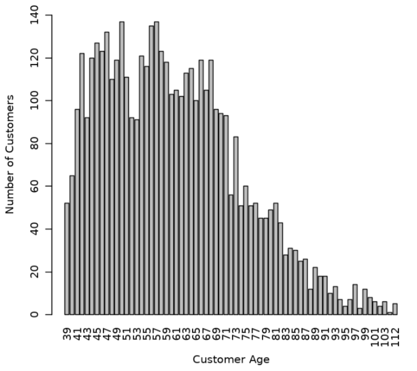
- View the data type of the columns in
CUST_DFwith the @desc operator, which is crucial for understanding to understand your data and perform calculations accurately.CUST_DF@desc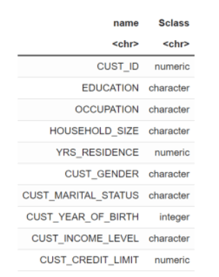
- To check if there are any missing values in the data, run the following code. The following code gives you the total number of missing values in the
CUST_DFproxy object.sum(is.na(CUST_DF)) 0The value 0 indicates that there are no missing values in the
CUST_DFproxy object. - Use the crosstab method to perform a cross-column analysis of the ore.frame object in the database. By default, it computes a frequency table for the columns unless a column and an aggregation function have been passed to it. In this example, the crosstab function displays the distribution of unique values of
CUST_CREDIT_LIMITalong the x-axis and its occurrence frequency along the y-axis.In the output, click the Bar chart. In the Settings tab, choose “CUST_CREDIT_LIMIT” as the Group By column, and use “Last” as the Aggregate Duplicates function.
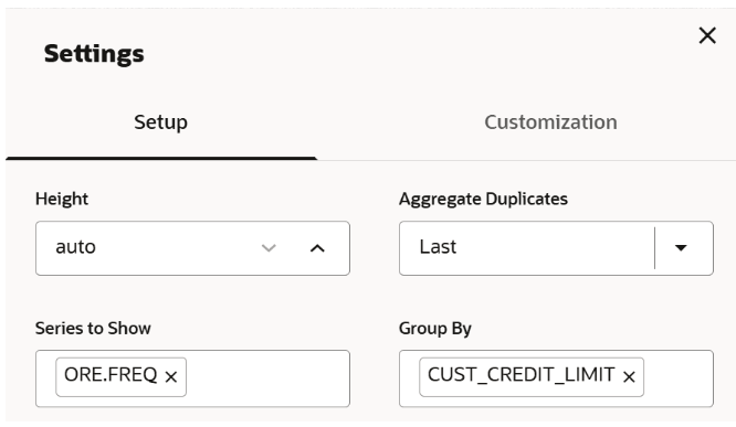
ct <- ore.crosstab(~CUST_CREDIT_LIMIT, data=CUST_DF)
z.show(ct)
- To compute the statistics of the
CUST_DFtable, use thesummaryfunction.options(width = 80) summary(subset(CUST_DF, select = -CUST_ID)) CUST_GENDER CUST_MARITAL_STATUS CUST_INCOME_LEVEL Length:4500 Length:4500 Length:4500 Class :ore.character Class :ore.character Class :ore.character Mode :character Mode :character Mode :character CUST_CREDIT_LIMIT HOUSEHOLD_SIZE YRS_RESIDENCE Y_BOX_GAMES Min. : 1500 Length:4500 Min. : 0.000 Min. :0.0000 1st Qu.: 5000 Class :ore.character 1st Qu.: 3.000 1st Qu.:0.0000 Median : 9000 Mode :character Median : 4.000 Median :0.0000 Mean : 7924 Mean : 4.022 Mean :0.3124 3rd Qu.:11000 3rd Qu.: 5.000 3rd Qu.:1.0000 Max. :15000 Max. :14.000 Max. :1.0000 CUST_AGE Min. : 39.00 1st Qu.: 49.00 Median : 59.00 Mean : 60.38 3rd Qu.: 69.00 Max. :112.00This completes the data understanding stage.
Data Preparation
Before building the model you want to clean the data, if needed. Usually, data can contain outliers that may form a separate cluster, which can affect model quality. The command below defines the function filter_outliers to calculate the interquartile range for a dataframe object. The function remove_outliers uses a for loop to compute the interquartile range for the list of features. The user-defined function remove_outliers uses the interquartile range to find outliers in the data and remove them.
# create filter outliers function
filter_outliers <- function(x) {

    # calculate first quantile
    Quantile1 <- quantile(x, probs=.25)

    # calculate third quantile
    Quantile3 <- quantile(x, probs=.75)

    # calculate inter quartile range
    IQR = Quantile3-Quantile1

    # return true or false
    x < Quantile3 + (IQR*1.5) & x > Quantile1 - (IQR*1.5)
}

# create remove outliers function
remove_outliers <- function(dataframe,
                            columns=names(dataframe)) {

    # for loop to traverse in columns vector
    for (col in columns) {

        # remove observation if it satisfies outlier function
        dataframe <- dataframe[filter_outliers(dataframe[[col]]),]
    }
    ore.pull(dataframe)
}

CUST_DF_CLEAN <- remove_outliers(CUST_DF, c('CUST_AGE', 'CUST_CREDIT_LIMIT', 'YRS_RESIDENCE', 'Y_BOX_GAMES'))
CUST_DF_CLEAN <- ore.push(CUST_DF_CLEAN)
dim(CUST_DF_CLEAN)

4233 9
This completes the data preparation stage.
Parent topic: Clustering Use Case
3.2.3 Build Model
To evaluate a model's performance, it is common practice to split the data into training and test sets. This allows you to assess how well the model generalizes to unseen data. However, in unsupervised learning, such as clustering, there are no labels or predictors available to calculate accuracy or evaluate performance. As a result, you can use the entire dataset to build the model without the need to split it. Since there is no ground truth to compare the results against, the training-test split is neither applicable nor useful in unsupervised learning.
Algorithm Selection
- K-Means (KM)
- Expectation-Maximization (EM)
- Orthogonal Partitioning Cluster (O-Cluster)
The k-Means(KM) algorithm is a distance-based clustering algorithm that partitions the data into a specified number of clusters. Distance-based algorithms are based on the concept that nearby data points are more related to each other than data points that are farther away. The algorithm iteratively tries to minimize the within-cluster variance with respect to its nearest cluster centroid. The Expectation-Maximization(EM) algorithm uses a probabilistic clustering based on a density estimation algorithm. The Orthogonal Partitioning Cluster (O-Cluster) algorithm is a density-based clustering method designed for large, high-dimensional datasets.
A good starting point for clustering is the K-means algorithm. It works by assigning each data point to the closest cluster center (centroid). Unlike some methods, K-means doesn't make assumptions about the underlying shapes of the clusters. This simplicity makes it a user-friendly choice for many applications, and it will be the method we use for this use case.
We will use the elbow method to determine the number of clusters in the dataset. The elbow method uses the leaf clusters. In cluster analysis, the elbow method is a heuristic used in determining the number of clusters in a data set. The method consists of plotting the variance (or dispersion) as a function of the number of clusters and picking the elbow of the curve as the number of clusters to use. We will start with one cluster, and continue specifying one cluster through 8 clusters. We will look for the "elbow" in the resulting dispersion curve to assess which number of clusters seems best.
To specify model settings and build a k-Means model object that will segment the data, run the following command. The settings are given as key-value or dictionary pairs where it refers to parameters name and value setting respectively. Here are some of the settings specified: KMNS_ITERATIONS, KMNS_RANDOM_SEED, KMNS_CONV_TOLERANCE, KMNS_NUM_BINS, KMNS_DETAILS, and PREP_AUTO. The k-Means algorithm uses the number of clusters (k) and other settings to configure the algorithm, as shown here:
settings = list(
    KMNS_ITERATIONS = 15,
    KMNS_RANDOM_SEED = 1,
    KMNS_CONV_TOLERANCE = 0.001,
    KMNS_NUM_BINS = 11,
    KMNS_DETAILS = "KMNS_DETAILS_HIERARCHY",
    CASE_ID_COLUMN_NAME = "CUST_ID"
)

KM.MOD <- ore.odmKMeans(
    formula = ~.-CUST_ID,
    data = CUST_DF_CLEAN,
    num.centers = 3,
    odm.settings = settings
)

KM.MOD
The following is the list of algorithm settings used in this example:
- KMNS_ITERATIONS: Specifies the maximum number of iterations for k-Means that are allowed. The default number of iterations is
20. - KMNS_RANDOM_SEED: The random number generator uses a number called the random seed to initialize itself. The random number generator generates random numbers that are used by the k-Means algorithm to select the initial cluster centroid. This setting controls the seed of the random generator used during the k-Means initialization. It must be a non-negative integer value. The default is 0.
- KMNS_CONV_TOLERANCE: Convergence Tolerance is the threshold value for the change in the centroids between consecutive iterations of the algorithm. This setting is used to specify the minimum Convergence Tolerance for k-Means. The algorithm iterates until the minimum Convergence Tolerance is satisfied or until the maximum number of iterations, specified in
KMNS_ITERATIONS, is reached. Decreasing the Convergence Tolerance produces a more accurate solution but may result in longer run times. The default Convergence Tolerance is0.001. - KMNS_NUM_BINS: Number of bins in the attribute histogram produced by k-Means. The bin boundaries for each attribute are computed globally on the entire training data set. The binning method is equi-width. All attributes have the same number of bins with the exception of attributes with a single value that have only one bin.
- KMNS_DETAILS: This setting determines the level of cluster details that is computed during the build. The value
KMNS_DETAILS_ALLmeans that the cluster hierarchy, record counts, and descriptive statistics (means, variances, modes, histograms, and rules) are computed and this is the default value. The valueKMNS_DETAILS_NONEmeans no cluster details are computed and only the scoring information persisted. The valueKMNS_DETAILS_HIERARCHYmeans cluster hierarchy and cluster record counts are computed. PREP_AUTO: Used to specify whether to use automatic data preparation or if the user is responsible for algorithm-specific data preparation. By default, it is enabled with a constant value as'PREP_AUTO':PREP_AUTO_ONand requires the DBMS_DATA_MINING package. Alternatively, it can also be specified as'PREP_AUTO': 'ON'.- ~.-CUST_ID: This argument is passed to the function to cluster the data in the
CUST_DF_CLEANdata frame, excluding theCUST_IDcolumn. - CUST_DF_CLEAN: The data frame that needs to be clustered.
num.centers: Defines the number of clusters for a clustering model. A value greater than or equal to 1. The default value is 10.- odm.settings: A list to specify in-database algorithm parameter settings. This argument is applicable to building a model in Database 12.2 or later. Each list element's name and value refer to the parameter setting name and value, respectively. The setting value must be numeric or string.
The output appears as follows:
Call:
ore.odmKMeans(formula = ~. - CUST_ID, data = CUST_DF_CLEAN, num.centers = 3,
    odm.settings = settings)

Settings:
                                               value
clus.num.clusters                                  3
block.growth                                       2
conv.tolerance                                 0.001
details                            details.hierarchy
distance                                   euclidean
iterations                                        15
min.pct.attr.support                             0.1
num.bins                                          11
random.seed                                        1
split.criterion                             variance
odms.details                             odms.enable
odms.missing.value.treatment odms.missing.value.auto
odms.sampling                  odms.sampling.disable
prep.auto                                         ON
Parent topic: Clustering Use Case
3.2.4 Deploy the Model
Here are several approaches to deploy your OML4R model and leverage its insights:
Prediction using R API:
This is the simplest method, ideal for quick analysis or prototyping. You can directly use the fitted model within your R environment to make predictions on new data.
pred <- predict(km.mod.ere, CUST_DF_CLEAN, supplemental.cols = "CUST_ID")

print(pred)  # View predictions for new data
Deploy model in different database:
For production deployments within the different database, leverage the built-in functionalities:
- Export: Use DBMS_DATA_MINING.EXPORT_SERMODEL to export the trained model (CUST_CLUSTER_MODEL_ERE) to a BLOB object in Database 1.
- Transfer: Move the BLOB object (e.g., BFile) to Database 2.
- Import: Use DBMS_DATA_MINING.IMPORT_SERMODEL in Database 2 to import the model from the transferred BLOB object.
Running a user-defined R function from R and SQL, and on ADB REST:
For periodic model updates with new data, create a user-defined R function:
- Define model settings (number of clusters, distance metric, etc.).
- Drop any existing model named CUST_CLUSTER_MODEL_ERE (optional).
- Train the model using ore.odmKMeans.
- Optionally, generate predictions for new data and display them.
Schedule this script to run periodically using Oracle's scheduling features.
Example 3-1 Defining the R function in the script repository and running it from R
#suppress warnings#
options(warn=-1)

build.km.1 <- function(){
    settings = list('KMNS_ITERATIONS'='10',
           'KMNS_DISTANCE'='KMNS_EUCLIDEAN',
           'KMNS_NUM_BINS'='10',
           'KMNS_DETAILS'='KMNS_DETAILS_ALL',
           'PREP_AUTO'='ON',
           'MODEL_NAME'='CUST_CLUSTER_MODEL_ERE')

    ore.exec(paste("BEGIN DBMS_DATA_MINING.DROP_MODEL('CUST_CLUSTER_MODEL_ERE'); EXCEPTION WHEN OTHERS THEN NULL; END;", sep=""))

    km.mod.ere <- ore.odmKMeans(~ . -CUST_ID, CUST_DF_CLEAN, num.centers=3, odm.settings=settings)

    # Show predictions
    pred <- predict(km.mod.ere, CUST_DF_CLEAN, supplemental.cols="CUST_ID")
    pred
}

ore.doEval(FUN = build.km.1)
The output appears as follows:

Example 3-2 Running the user-defined R script from SQL
--set the access token
exec rqSetAuthToken('<access token>');

--run user-defined R script from SQL
SELECT *
  FROM table(
    rqEval2(
         NULL,
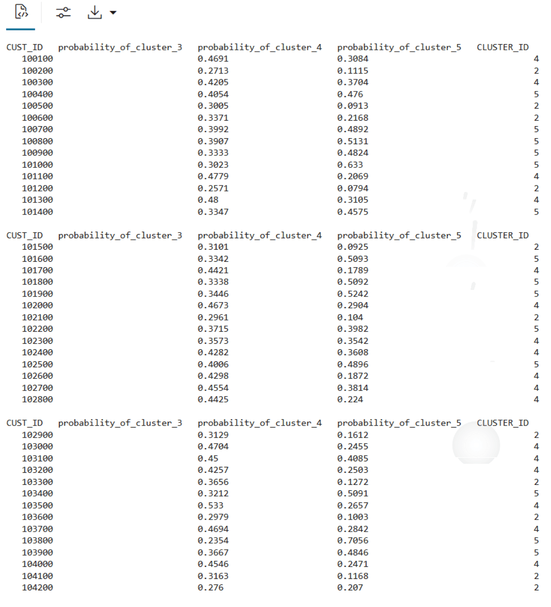
        '{"CUST_ID": "NUMBER", "probability_of_cluster_3": "BINARY_DOUBLE", "probability_of_cluster_4": "BINARY_DOUBLE",
          "probability_of_cluster_5": "BINARY_DOUBLE", "CLUSTER_ID": "NUMBER"}',
        'build.km.1'));
The SQL output appears as follows:
Example 3-3 Running the R script from ADB REST using CURL command:
curl -i -X POST --header "Authorization: Bearer ${token}" \
--header 'Content-Type: application/json' --header 'Accept: application/json' \
-d '{}' \
"<oml-cloud-service-location-url>/oml/api/r-scripts/v1/do-eval/build.km.1"
The REST response appears as follows:
{

    "result": [

        {

            "probability_of_cluster_5": 0.3084,

            "CUST_ID": 100100,

            "probability_of_cluster_4": 0.4691,

            "'2'": 0.2224,

            "CLUSTER_ID": 4

        },

        {

            "probability_of_cluster_5": 0.1115,

            "CUST_ID": 100200,

            "probability_of_cluster_4": 0.2713,

            "'2'": 0.6172,

            "CLUSTER_ID": 2

        },

        ……

        {

            "probability_of_cluster_5": 0.3974,

            "CUST_ID": 104498,

            "probability_of_cluster_4": 0.4256,

            "'2'": 0.177,

            "CLUSTER_ID": 4

        },

        {

            "probability_of_cluster_5": 0.273,

            "CUST_ID": 104499,

            "probability_of_cluster_4": 0.4102,

            "'2'": 0.3168,

            "CLUSTER_ID": 4

        }

    ]

}
Persistent Table for SQL Integration:
There are two different approaches for creating persistent data structures: a dynamic view ('CUST_DF_VIEW') for accessing the latest data and a materialized table ('CUST_DF_CLEAN') for capturing a snapshot of the data.
Example 3-4 Creating a persistent data structure using a dynamic view
- Use the following code to create a view
ore.drop(view="CUST_DF_VIEW") ore.create(CUST_DF,view="CUST_DF_VIEW") - Use the following SQL query to create a view named
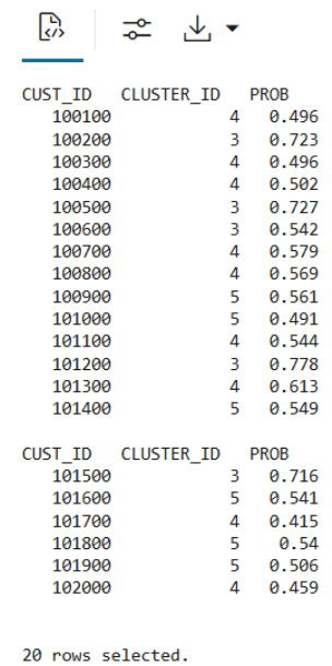
KM_PRED_VIEW. This view will dynamically score data based on the existing viewCUST_DF_VIEW.CREATE OR REPLACE VIEW KM_PRED_VIEW AS SELECT CUST_ID, CLUSTER_ID(CUST_CLUSTER_MODEL_ERE USING *) AS CLUSTER_ID, round (CLUSTER_PROBABILITY (CUST_CLUSTER_MODEL_ERE USING *),3) AS PROB FROM CUST_DF_VIEW; - Use the following code to display first 20 rows of dynamic scoring view 'KM_PRED_VIEW'
select * from KM_PRED_VIEW
where rownum < 21;
The output appears as follows:
Example 3-5 Creating a persistent data structure using a materialized table
- Use the following code to create a table named
CUST_DF_CLEANto store the cleaned data in the database.ore.drop(table="CUST_DF_CLEAN") ore.create(CUST_DF_CLEAN,table="CUST_DF_CLEAN") - Use the following code to create a table named
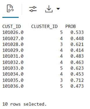
KM_SCORE_TABLE, which will store a static snapshot of the scoring results based on the data in theCUST_DF_CLEANtable.DROP TABLE KM_SCORE_TABLE; CREATE TABLE KM_SCORE_TABLE AS SELECT CUST_ID, CLUSTER_ID(CUST_CLUSTER_MODEL_ERE USING *) AS CLUSTER_ID, round(CLUSTER_PROBABILITY (CUST_CLUSTER_MODEL_ERE USING *),3) AS PROB FROM CUST_DF_CLEAN; - Use the following code to display the first 10 rows of the scoring snapshot table.
select * from KM_SCORE_TABLE where rownum <= 10;The output appears as follows:
- Use the SQL Interface for scoring and then visualize the results using OML Notebooks.
Use the following code to query the table, apply the CLUSTER_SET function for prediction, and extract details from the model output using XML parsing.
SELECT CUST_ID,
       CLUSTER_ID,
       ROUND(PROB*100,0) PROB_PCT,
       RTRIM(TRIM(SUBSTR(OUTPRED."Attribute1",17,100)),'rank="1"/>') FIRST_ATTRIBUTE,
       RTRIM(TRIM(SUBSTR(OUTPRED."Attribute2",17,100)),'rank="2"/>') SECOND_ATTRIBUTE,
       RTRIM(TRIM(SUBSTR(OUTPRED."Attribute3",17,100)),'rank="3"/>') THIRD_ATTRIBUTE
FROM (SELECT CUST_ID, S.CLUSTER_ID, PROBABILITY PROB,
             CLUSTER_DETAILS(KM_CLUSTERING_MODEL USING T.*) DETAIL
      FROM (SELECT V.*, CLUSTER_SET(KM_CLUSTERING_MODEL, NULL, 0.2 USING *) PSET
            FROM CUST_DF_KM V
            WHERE cust_id = ${CUST_ID ='101362','101362'|'102087'| '100456'}) T,
                  TABLE(T.PSET) S
            ORDER BY 2 DESC) OUT,
            XMLTABLE('/Details'
                      PASSING OUT.DETAIL
                      COLUMNS
                      "Attribute1" XMLType PATH 'Attribute[1]',
                      "Attribute2" XMLType PATH 'Attribute[2]',
                      "Attribute3" XMLType PATH 'Attribute[3]') OUTPRED
The output appears as follows:

Parent topic: Clustering Use Case