3.3 Time Series Use Case
You work in an electronics store, and sales of laptops and tablets have increased over the past two quarters. You want to forecast product sales for the next four quarters using historical timestamped data. To do this, you apply the Exponential Smoothing algorithm, which predicts future sales by analyzing patterns over evenly spaced time intervals in the historical data.
Table 3-1 Related Content
| Topic | Link |
|---|---|
| About Time Series | About Time Series |
| About Model Setting | About Model Setting |
| Shared Settings | Shared Settings |
| Time Series Algorithm | Time Series Algorithm |
Before you start your OML4R use case journey, ensure that you have the following:
-
Data Set
The data set used for this use case is from the SH schema. The SH schema can be readily accessed in Oracle Autonomous AI Database. For on-premises databases, the schema is installed during the installation or can be manually installed by downloading the scripts. See Installing the Sample Schemas.
You will use the
SALEStable from theSHschema. You can access the table by running theSELECTstatements in OML Notebooks. -
Database
Select or create a database using one of the following options:
- Get your FREE cloud account. Go to https://cloud.oracle.com/database and select Oracle Database Cloud Service (DBCS), or Oracle Autonomous AI Database. Create an account and create an instance. See Autonomous Database Quick Start Workshop.
- Download the latest version of Oracle Database (on premises).
-
Machine Learning Tools
Use OML Notebooks for Oracle Autonomous AI Database.
Topics:
- Access Data
Access the data set from the SH Schema and explore the data to understand the attributes. - Explore Data
Explore the data to understand its structure and assess its quality. At this stage, identify the data types and detect any noise present. Check for missing values as well as numeric outliers. - Build Model
To build a model using time series data, apply the Exponential Smoothing algorithm to the proxy objectESM_SH_DATAcreated during the exploratory stage. - Evaluate
Evaluate your model by reviewing diagnostic metrics and performing quality checks.
Related Topics
Parent topic: Use Cases
3.3.1 Access Data
Access the data set from the SH Schema and explore the data to understand the attributes.
Remember:
The data set used for this use case is from the SH schema. The SH schema can be readily accessed in Oracle Autonomous AI Database. For on-premises databases, the schema is installed during the installation or can be manually installed by downloading the scripts. See Installing the Sample Schemas.
- Access the data.
- Examine the various attributes or columns of the data set.
- Assess data quality (by exploring the data).
Access Data
You will be using the SALES table data from the SH schema.
Examine Data
The following table displays information about the attributes from
SALES:
| Attribute Name | Information |
|---|---|
PROD_ID |
The ID of the product |
CUST_ID |
The ID of the customer |
TIME_ID |
The timestamp of the purchase of the product in yyy-mm-dd hh:mm:ss format |
CHANNEL_ID |
The channel ID of the channel sales data |
PROMO_ID |
The product promotion ID |
QUANTITY_SOLD |
The number of individual units or items sold. |
AMOUNT_SOLD |
The total monetary value of the sales (i.e., the revenue generated) |
Identify Target Variable
In this use case, the task is to build a model that predicts the amount sold. Therefore, the target variable is the attribute AMOUNT_SOLD.
Parent topic: Time Series Use Case
3.3.2 Explore Data
Explore the data to understand its structure and assess its quality. At this stage, identify the data types and detect any noise present. Check for missing values as well as numeric outliers.
Note:
Each record in the database is called a case, and each case is identified by a case_id. Here, the case id is TIME_ID, which serves as the independent variable. You are forecasting sales over evenly spaced time intervals.
The following steps will guide you through exploratory data analysis.
-
Import libraries
Run the following command in an R interpreter paragraph (using %r) in a notebook to import the Oracle Machine Learning for R libraries and suppress warnings regarding row ordering. This establishes a default connection to the database for use by OML4R.Note:
The OML4R functions are prefixed with "ore," which refers to the original product name "Oracle R Enterprise."library(ORE) options(ore.warn.order=FALSE) -
Create a DataFrame proxy object on the SH.SALES table
Use the
This script uses the ore.sync function to create a data.frame proxy object to the table SH.SALES in the object ESM_SALES. It then attaches the synchronized object to the R environment withore.syncfunction to create the a proxy objectESM_SALESfor theSH.SALESdatabase table. Theore.syncfunction returns anore.frameobject that represents the table in OML4R.ore.attach(), allowing direct access toESM_SALESas if it were a local data frame. Finally, it displays the first few rows of this data usinghead()combined with ORE’s formatted output functionz.show().ore.sync(query = c(ESM_SALES = "select * from SH.SALES")) ore.attach() z.show(head(ESM_SALES))The output appears as follows:

This output displays the first 6 rows of the
SH.SALESdatabase table, including all available columns. It allows you to quickly inspect a sample of the sales data stored in the Oracle AI Database directly from your OML4R session. -
Sales dataset row and column count
To determine the number of rows and columns in the
ore.frameobjectSALES, use the functiondim(SALES).This script runs an R command inside a notebook to return the number of rows and columns of the
ESM_SALESdata frame or table.%r dim(ESM_SALES)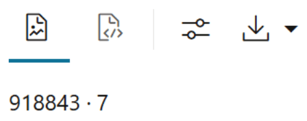
The output shows the number of rows and columns in the
ESM_SALESdataset to understand the shape and scale of the data you are working with in OML4R. -
Sales Dataset Column Types
Use the following code to view the data type of each column.
This script retrieves and displays metadata for the
ESM_SALESobject in OML4R, providing details about the structure and columns of the linked Oracle AI Database table.
The output appears as follows:%r ESM_SALES@desc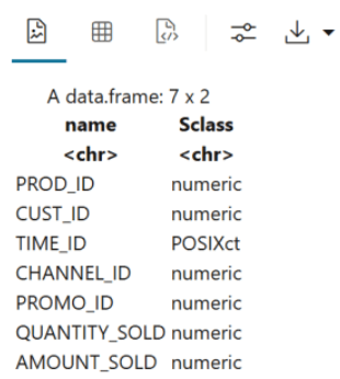
The output of
ESM_SALES@descis a structure of theESM_SALESobject. It includes Column names and Data types. -
Count of missing values by column
To check if there are any missing values in the data, run the following code. It returns you the total number of missing values in the
ESM_SALESproxy object to assess data completeness.%r sum(is.na(ESM_SALES))The output appears as 0, which indicates that there are no missing values in the
ESM_SALESproxy object. -
Prepare the data for sales forecasting, start by selecting the required columns from the
SH.SALEStable.Use the
ore.sync()function to create a proxy object namedSALES_TIME_AMOUNTcontaining theTIME_IDandAMOUNT_SOLDcolumns..This defines a new
ore.data.frameobject in R calledSALES_TIME_AMOUNTby linking it to a query that selectsTIME_IDandAMOUNT_SOLDcolumns from theSH.SALEStable in an Oracle AI Database. It helps in-database analytics without fully loading the data into R.%r ore.sync(query = c(SALES_TIME_AMOUNT = "select TIME_ID, AMOUNT_SOLD from SH.SALES")) z.show(head(SALES_TIME_AMOUNT)))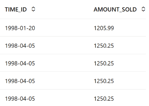 The output shows the formatted table with the first 6 rows of the SALES_TIME_AMOUNT dataset. It includes two columns:
- TIME_ID – A time identifier (date).
- AMOUNT_SOLD – A numeric value showing the amount sold for each transaction.
-
Use the
dim()function to view the dimensions (number of rows and columns) of theSALES_TIME_AMOUNTproxy object. This helps confirm the size of the dataset retrieved from theSH.SALEStable.The returns the number of rows and columns in the
SALES_TIME_AMOUNTdataset, showing you the shape of the data queried from the database.%r dim(SALES_TIME_AMOUNT)
The output of
dim(SALES_TIME_AMOUNT)shows that the dataset contains 918843 rows and 2 columns. This gives you a quick understanding of the dataset’s size and structure.
This gives you a quick understanding of the dataset’s size and structure.
Parent topic: Time Series Use Case
3.3.3 Build Model
To build a model using time series data, apply the Exponential Smoothing algorithm to the proxy object ESM_SH_DATA created during the exploratory stage.
Oracle provides the Exponential Smoothing algorithm specifically for time series forecasting.
- Trend refers to the long-term increase or decrease in the data over time. It captures the general direction or movement of the series, whether upward, downward, or stable.
- Seasonality refers to regular, repeating patterns or cycles in the data that occur at fixed intervals, such as daily, monthly, or quarterly fluctuations caused by factors like holidays, weather, or business cycles.
In the additive form, the amplitude of variation (the size of the repeating seasonal fluctuations) is independent of the overall level of the time series, whereas in the multiplicative form, the seasonal variation changes proportionally with the level. Here, level refers to the baseline value or the underlying magnitude of the time series at a given point in time. This suggests a multiplicative model, where seasonal fluctuations are proportional to the level of the series—larger when the overall values are high and smaller when the values are low. Additive models assume that the error (or noise), trend, and seasonality are linear components. These components combine in a recursive way to form the final model.
To build a model using a supervised learning approach, it is common to split the dataset into training and test sets. However, time series modeling differs from classification and regression in that it predicts the next value in a series based on the preceding items in the series. In this case, splitting the dataset is unnecessary because the model always forecasts the current value using only past data. Although it may appear that the model is trained and tested on the same data, each forecast is based solely on prior time points.
In this use case, you will use the proxy object ESM_SH_DATA to build the Exponential Smoothing model.
- To get help on the Exponential Smoothing Model (ESM), run the following script:
%r

help(ore.odmESM)
The output of
help(ore.odmESM)is the function reference for theore.odmESM. It guides you on how to use it to build exponential smoothing models for time series forecasting using in-database analytics in Oracle. This is helpful for learning the syntax, understanding parameters, and seeing example usage. - Create a Holt-Winters model using the quarterly setting. The Holt-Winters model is a way to predict future values in a time series by looking at patterns like trends (overall direction) and seasonality (regular ups and downs). It updates its predictions step-by-step using only past data, never looking ahead.
To build the model using the
ESM_SH_DATAproxy object, run the following statement:This script deletes any existing model named
ESM_SALES_FORECAST_1, then trains a Holt-Winters exponential smoothing model to forecastAMOUNT_SOLDon a quarterly basis for the next 4 quarters. It uses in-database modeling usingore.odmESM, and stores the trained model in the objectMODfor further use.%r ore.drop(model = 'ESM_SALES_FORECAST_1') settings = list(EXSM_INTERVAL = 'EXSM_INTERVAL_QTR', EXSM_PREDICTION_STEP = 4, EXSM_MODEL = 'EXSM_HW', EXSM_SEASONALITY = 4, EXSM_ACCUMULATE = 'EXSM_ACCU_TOTAL', MODEL_NAME='ESM_SALES_FORECAST_1', case_id_column_name = "TIME_ID") MOD <- ore.odmESM(AMOUNT_SOLD~., SALES_TIME_AMOUNT, odm.settings= settings)Examine the script:
EXSM_INTERVAL: Specifies the interval of the dataset or the unit of interval size, such as day, week, month, etc. This setting applies only to the time column of datetime type. For example, if you want to predict quarterly sales, set this toEXSM_INTERVAL_QTR.EXSM_PREDICTION_STEP: Specifies how many future predictions to make. For example, if you want to predict one value per quarter, setting this to4will generate predictions for four quarters into the future.EXSM_MODEL: Specifies the type of exponential smoothing model to be used. As an example,EXSM_WINTERSrepresents the Holt-Winters triple exponential smoothing model with additive trend and multiplicative seasonality. This type of model considers various combinations of additive and multiplicative trend, seasonality and error, with and without trend damping.- Additive trend: A trend where the increase or decrease in values happens by adding a constant amount over time.
- Multiplicative trend: A trend where values grow or shrink by multiplying by a constant factor over time (e.g., percentage growth).
- Seasonality: Refers to regular, repeating patterns or fluctuations in a time series that happen at specific intervals—like daily, weekly, monthly, or yearly.
- Error components: The random noise or unexplained fluctuations in the data that aren’t captured by trend or seasonality.
- Trend damping: A technique that slows down (reduces) the trend growth or decline over time, preventing it from continuing indefinitely at the same rate.
EXSM_SEASONALITY: This parameter specifies the length of the seasonal cycle and must be a positive integer greater than 1. For example, if the value is 4, it means the seasonal pattern repeats every 4 time periods—such as the four quarters in a year. In this case, each group of four consecutive values represents one complete seasonal cycle.EXSM_SETMISSING: Specifies how to handle missing values. The special valueEXSM_MISS_AUTOindicates that if the time series contains missing values, it should be treated as an irregular time series.
This completes the model building stage.
Parent topic: Time Series Use Case
3.3.4 Evaluate
Evaluate your model by reviewing diagnostic metrics and performing quality checks.
In some cases, querying dictionary views and model detail views may be sufficient to assess model performance. However, for a more thorough evaluation, you can compute test metrics such as Conditional Log-Likelihood, Average Mean Squared Error (AMSE), Akaike Information Criterion (AIC), and others.
Model Settings Information
Evaluate the model by examining the various statistics generated after model creation. These statistics provide insights into the model's quality.
%r

summary(MOD)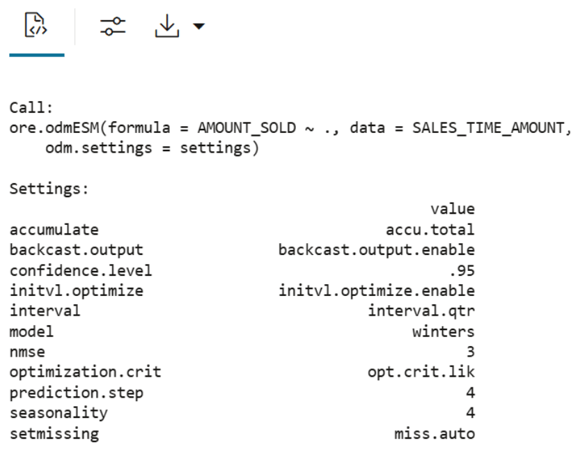
This script outputs a summary of a created exponential smoothing model, trained in the Oracle AI Database using the SALES_TIME_AMOUNT data. The summary confirms model type, input variables, target, forecast settings, and Oracle model metadata — all stored in the object MOD and available in the database as ESM_SALES_FORECAST_1.
Forecast
In this step, you will forecast sales for the next four quarters.
-
Forecast AMOUNT SOLD
The model
ESM_MODpredicts four future values of AMOUNT_SOLD, along with lower and upper confidence bounds. The results are sorted in descending time order, displaying the most recent forecasted points first.%r modelDetails <- summary(MOD) PRED <- modelDetails$predictions z.show(ore.sort(PRED, by='CASE_ID', reverse=TRUE))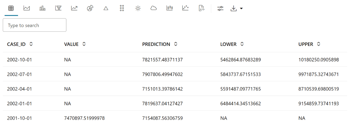
The output is a table showing the forecasted values of
AMOUNT_SOLDfor the next 4 futureCASE_IDperiods (For example: quarters), sorted in descending order of time. This helps you view the most recent predictions at the top, providing a clear snapshot of expected future sales.Explanation of each column in the output:
- CASE_ID:
A unique identifier for each input record (or row) used during prediction. Helps track which prediction corresponds to which original data row.
- Value:
The actual (observed) value from the dataset, typically the true target/output variable.
- Prediction:
The predicted value generated by the model for that record. This can be a class label (for classification) or a numeric value (for regression).
- Lower:
The lower bound of the confidence or prediction interval. Indicates the lowest expected value with a given level of confidence (e.g., 95%).
- Upper:
The upper bound of the confidence or prediction interval. Indicates the highest expected value with a given level of confidence.
- CASE_ID:
-
Chart Forecasted AMOUNT_SOLD Values with Confidence Intervals
To visualize the forecasted values in OML Notebooks, run the same query as above with the following chart settings:
z.show(ESM_MOD.prediction.sort_values(by='TIME_SEQ'))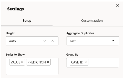

The line chart effectively illustrates how the model’s predictions track the actual observed values (Value) over time (time_id).
This completes the prediction step. The model has successfully forecasted sales for the next four quarters. These forecasts help track sales trends and provide valuable insights for inventory planning.
Parent topic: Time Series Use Case