k-Means

7.12 k-Means

The ore.odmKM function uses the in-database k-Means (KM) algorithm, a distance-based clustering algorithm that partitions data into a specified number of clusters.

The algorithm has the following features:

Several distance functions: Euclidean, Cosine, and Fast Cosine distance functions. The default is Euclidean.
For each cluster, the algorithm returns the centroid, a histogram for each attribute, and a rule describing the hyperbox that encloses the majority of the data assigned to the cluster. The centroid reports the mode for categorical attributes and the mean and variance for numeric attributes.

For information on the ore.odmKM function arguments, call help(ore.odmKM).

Settings for a k-Means Models

The following table lists settings that apply to k-Means models.

Table 7-11 k-Means Model Settings

Setting Name	Setting Value	Description
`KMNS_CONV_TOLERANCE`	`TO_CHAR(0 < X < 1)`	Minimum Convergence Tolerance for k-Means. The algorithm iterates until the minimum Convergence Tolerance is satisfied or until the maximum number of iterations, specified in `KMNS_ITERATIONS`, is reached. Decreasing the Convergence Tolerance produces a more accurate solution but may result in longer run times. The default Convergence Tolerance is `0.001`.
`KMNS_DISTANCE`	`KMNS_COSINE` `KMNS_EUCLIDEAN`	Distance function for k-Means. The default distance function is `KMNS_EUCLIDEAN`.
`KMNS_ITERATIONS`	`TO_CHAR(X > 0)`	Maximum number of iterations for k-Means. The algorithm iterates until either the maximum number of iterations is reached or the minimum Convergence Tolerance, specified in `KMNS_CONV_TOLERANCE`, is satisfied. The default number of iterations is `20`.
`KMNS_MIN_PCT_ATTR_SUPPORT`	`TO_CHAR(0 <= X <= 1)`	Minimum percentage of attribute values that must be non-null in order for the attribute to be included in the rule description for the cluster. If the data is sparse or includes many missing values, a minimum support that is too high can cause very short rules or even empty rules. The default minimum support is `0.1`.
`KMNS_NUM_BINS`	`TO_CHAR(X > 0)`	Number of bins in the attribute histogram produced by k-Means. The bin boundaries for each attribute are computed globally on the entire training data set. The binning method is equi-width. All attributes have the same number of bins with the exception of attributes with a single value that have only one bin. The default number of histogram bins is `11`.
`KMNS_SPLIT_CRITERION`	`KMNS_SIZE` `KMNS_VARIANCE`	Split criterion for k-Means. The split criterion controls the initialization of new k-Means clusters. The algorithm builds a binary tree and adds one new cluster at a time. When the split criterion is based on size, the new cluster is placed in the area where the largest current cluster is located. When the split criterion is based on the variance, the new cluster is placed in the area of the most spread-out cluster. The default split criterion is the `KMNS_VARIANCE`.
`KMNS_RANDOM_SEED`	`X >= 0`	This setting controls the seed of the random generator used during the k-Means initialization. It must be a non-negative integer value. The default is `0`.
`KMNS_DETAILS`	`KMNS_DETAILS_NONE` `KMNS_DETAILS_HIERARCHY` . `KMNS_DETAILS_ALL`	This setting determines the level of cluster detail that are computed during the build. `KMNS_DETAILS_NONE`: No cluster details are computed. Only the scoring information is persisted. `KMNS_DETAILS_HIERARCHY`: Cluster hierarchy and cluster record counts are computed. `KMNS_DETAILS_ALL`: Cluster hierarchy, record counts, descriptive statistics (means, variances, modes, histograms, and rules) are computed. This is the default value.
`KMNS_WINSORIZE` Note: Available only in Oracle Database 23ai.	`KMNS_WINSORIZE_ENABLE` `KMNS_WINSORIZE_DISABLE`	To winsorize data, enable or disable this parameter. Data is restricted in a window size of six standard deviations around the mean value when winsorize is enabled. This functionality can be used with `AUTO_DATA_PREP` turned `ON` and `OFF`. The values outside the range are replaced with the ends of the interval. Winsorize is not enabled by default. Note: Winsorize is only available when the `KMNS_EUCLIDEAN` distance function is used. An exception is raised if Winsorize is enabled and other distance functions are set.

Example 7-14 Using the ore.odmKMeans Function

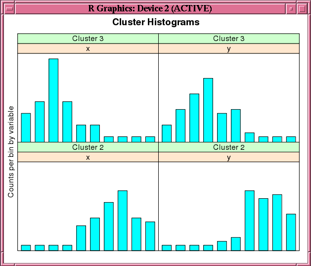
This example demonstrates the use of the ore.odmKMeans function. The example creates two matrices that have 100 rows and two columns. The values in the rows are random variates. It binds the matrices into the matrix x, then coerces x to a data.frame and pushes it to the database as x_of, an ore.frame object. The example next calls the ore.odmKMeans function to build the KM model, km.mod1. It then calls the summary and histogram functions on the model. Figure 7-2 shows the graphic displayed by the histogram function.

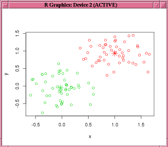
Finally, the example makes a prediction using the model, pulls the result to local memory, and plots the results.Figure 7-3 shows the graphic displayed by the points function.

x <- rbind(matrix(rnorm(100, sd = 0.3), ncol = 2),
           matrix(rnorm(100, mean = 1, sd = 0.3), ncol = 2))
colnames(x) <- c("x", "y")
x_of <- ore.push (data.frame(x))
km.mod1 <- NULL
km.mod1 <- ore.odmKMeans(~., x_of, num.centers=2)
summary(km.mod1)
histogram(km.mod1)
# Make a prediction.
km.res1 <- predict(km.mod1, x_of, type="class", supplemental.cols=c("x","y"))
head(km.res1, 3)
# Pull the results to the local memory and plot them.
km.res1.local <- ore.pull(km.res1)
plot(data.frame(x=km.res1.local$x, y=km.res1.local$y),
                col=km.res1.local$CLUSTER_ID)
points(km.mod1$centers2, col = rownames(km.mod1$centers2), pch = 8, cex=2)
head(predict(km.mod1, x_of, type=c("class","raw"),
             supplemental.cols=c("x","y")), 3)

Listing for This Example

R> x <- rbind(matrix(rnorm(100, sd = 0.3), ncol = 2),
+             matrix(rnorm(100, mean = 1, sd = 0.3), ncol = 2))
R> colnames(x) <- c("x", "y")
R> x_of <- ore.push (data.frame(x))
R> km.mod1 <- NULL
R> km.mod1 <- ore.odmKMeans(~., x_of, num.centers=2)
R> summary(km.mod1)
 
Call:
ore.odmKMeans(formula = ~., data = x_of, num.centers = 2)
 
Settings: 
                         value
clus.num.clusters            2
block.growth                 2
conv.tolerance            0.01
distance             euclidean
iterations                   3
min.pct.attr.support       0.1
num.bins                    10
split.criterion       variance
prep.auto                   on
 
Centers: 
            x           y
2  0.99772307  0.93368684
3 -0.02721078 -0.05099784
R> histogram(km.mod1)
R> # Make a prediction.
R> km.res1 <- predict(km.mod1, x_of, type="class", supplemental.cols=c("x","y"))
R> head(km.res1, 3)
            x          y CLUSTER_ID
1 -0.03038444  0.4395409          3
2  0.17724606 -0.5342975          3
3 -0.17565761  0.2832132          3
# Pull the results to the local memory and plot them.
R> km.res1.local <- ore.pull(km.res1)
R> plot(data.frame(x=km.res1.local$x, y=km.res1.local$y),
+                  col=km.res1.local$CLUSTER_ID)
R> points(km.mod1$centers2, col = rownames(km.mod1$centers2), pch = 8, cex=2)
R> head(predict(km.mod1, x_of, type=c("class","raw"),
                supplemental.cols=c("x","y")), 3)
           '2'       '3'           x          y CLUSTER_ID
1 8.610341e-03 0.9913897 -0.03038444  0.4395409          3
2 8.017890e-06 0.9999920  0.17724606 -0.5342975          3
3 5.494263e-04 0.9994506 -0.17565761  0.2832132          3

Figure 7-2 shows the graphic displayed by the invocation of the histogram function in Example 7-14.

Figure 7-2 Cluster Histograms for the km.mod1 Model

Description of "Figure 7-2 Cluster Histograms for the km.mod1 Model"

Figure 7-3 shows the graphic displayed by the invocation of the points function in Example 7-14.

Figure 7-3 Results of the points Function for the km.mod1 Model

Description of "Figure 7-3 Results of the points Function for the km.mod1 Model"

Parent topic: OML4R Classes That Provide Access to In-Database Machine Learning Algorithms