Data Preparation

This stage focuses on building a clear understanding of the dataset through the following steps:

• Redundant Columns:
  • Clean the Data: Identify and remove duplicate records, redundant columns, and highly correlated columns.
• Data Subset Creation: Filter/select relevant columns.
• Visualizations: Generate visual representations to understand data patterns and relationships.
• Feature Engineering: Create new features like "Decade Built", "Sale Age", and "Street Address".
• Clean the DataFrame: Handle missing values, outliers, and inconsistencies.
• Dataframe Dimensions: Ensure correct dimensions after cleaning.

These steps provide a solid foundation for data preparation.

Redundant Columns: Cleaning Up the Data

To identify redundant columns, compare column names and descriptions for clues. Then analyze the data within the columns to see if the values are identical or highly correlated. Once you identify the redundant columns, you need to decide which one to remove. The column with more missing values, inconsistent formatting, or mostly a unique value can be removed.

Analyze Columns with Similar Naming Conventions

Analyse and compare pairs or groups of columns that appear similar due to their content or variations in naming conventions or formatting. The goal is to ensure data consistency, detect redundancy, and verify if columns represent the same information.

The following columns are compared:

• borough, Borough, and BoroCode
• YearBuilt and year_built
• ZipCode and zip_code

Similarly, this can be applied to other columns, such as building_class, BldgClass and building_class_at_sale; Address and address; etc.

1. Compare columns: borough, Borough, and BoroCode

   The column names “borough,” “Borough,” and “BoroCode” are quite similar, suggesting they may contain the same information. To verify this, print five random samples from each column for comparison. Additionally, based on the column descriptions, all three columns represent the Brooklyn borough, with values such as “BK” or “3.0.” Since the data is specific to Brooklyn, these columns are redundant and can be safely removed from the dataset.

   
   z.show(BROOKLYN[['borough','Borough', 'BoroCode']].sample(n=5))

   
   

   

   
   

2. Identify Matching Data Percentage

   def matching_percentage(data, cols, threshold=0.9):
       # Filter rows where both columns have non-zero values
       filtered_df = data[(data[cols[0]] != 0) & (data[cols[1]] != 0)]
       
       # Calculate matching percentage
       total_rows = len(filtered_df)
       matching_rows = len(filtered_df[filtered_df[cols[0]] == filtered_df[cols[1]]])
       matching_percentage = matching_rows / total_rows if total_rows else 0
       
       # Output result
       if matching_percentage >= threshold:
           print(f"The columns have a high percentage ({matching_percentage * 100:.2f}%) of matching values, suggesting similarity.")
       else:
           print("The columns do not have a high percentage of matching values.")

3. Compare columns: YearBuilt and year_built

   The column names "YearBuilt" and "year_built" are quite similar, suggesting they may contain the same information. To verify this, we should print out 5 random samples from each column.

   
   matching_percentage(BROOKLYN, ['YearBuilt', 'year_built'])

   The columns have a high percentage (99.25%) of matching values, suggesting
   similarity.

   The columns "YearBuilt", "year_built" contain similar information,so remove one. Remove "year_built" from the dataset.

4. Compare columns: ZipCode and zip_code

   
   matching_percentage(BROOKLYN, ['ZipCode', 'zip_code'])

   The columns have a high percentage (98.72%) of matching values, suggesting
   similarity.

   The column names "ZipCode" and "zip_code" are quite similar, suggesting they may contain the same information. To verify this, we should print out 5 random samples from each column.

   
   z.show(BROOKLYN[['ZipCode', 'zip_code']].sample(n=5))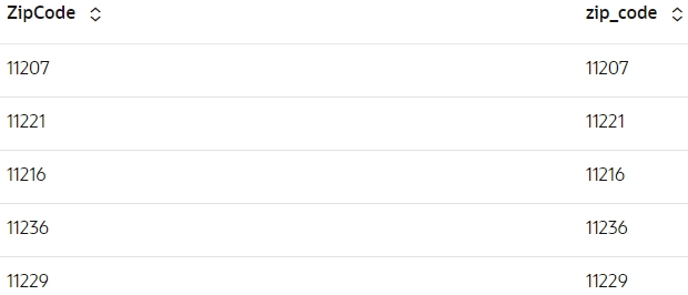

   
   

   

   
   

Filter data by selecting the desired columns

To focus on more reliable data, only houses built after the 1800s are included in the dataset. This is because houses built before the 1800s frequently have a single YearBuilt value of 0, indicating potentially missing or inaccurate information and more is exaplained in the next step.

BROOKLYN2 = BROOKLYN[(BROOKLYN['YearBuilt']>= 1800)][['building_class_at_sale', 'HealthCent', 'YearBuilt', 'ResidFAR', 
'sale_date', 'building_class_category', 'GarageArea', 'CD', 'YearAlter1', 'ID', 'SchoolDist', 'SanitDistr', 'PolicePrct','address',
'CT2010', 'commercial_units', 'BldgArea','NumFloors', 'sale_price','AssessTot', 'ResArea','land_sqft','LotFront', 
'LotArea','AssessLand', 'SHAPE_Area','year_of_sale', 'gross_sqft','XCoord','YCoord', 'SHAPE_Leng']]

# Dataframe dimension
BROOKLYN2.shape

(295356, 31)

Feature Engineering and Visualization

Create new columns and modify existing features based on insights gathered from visualizations. The newly engineered features are then merged back into the dataset to enhance its quality and readiness for modeling.

1. Built periods and their counts:

   • Analyze the distribution of the periods in which the houses were built and identify the least and most common periods within our dataset. The column, YearBuilt, is first rounded to the nearest integer value. These rounded values will then be categorized into predefined intervals, or bins. Count the number of YearBuilt within each bin to determine the frequency distribution of built periods.

     built_period = (BROOKLYN2['YearBuilt'] // 10) * 10 + oml.Integer(BROOKLYN2['YearBuilt'] % 10 >= 5) * 10
     bins_str = built_period.cut(bins=[1700,1800,1880,1900,1920,1940,1960,1980,2000,2020,2040])
     bins = sorted(bins_str.drop_duplicates().pull())
      
     z.show(pd.DataFrame({'Built Period':bins, 'Count':[oml.Integer(bins_str == b).sum() for b in bins]}))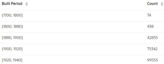

     
     
     
     
     

   • Visualisation of built periods and their counts

     # Data might be incomplete when DECADE_BUILT < 1900
      
     Nbins = 141
     n, bins, patches = plt.hist(built_period.pull(), Nbins)
     plt.xlabel('Built_Period')
     plt.ylabel('number of records')
     plt.yscale('log')
     p = plt.xlim(1795, 2025)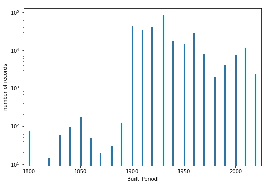

     
     
     
     
     

2. Preview sale price and count by binning

   • Analyze the distribution of the sale price of the houses and identify the least and most common sale price within our dataset. The column, sale_price, is rounded and then are categorized into predefined intervals, or bins. Count the number of sale_price within each bin to determine the frequency distribution of sale_price.

     Sale_Price=(BROOKLYN2['sale_price'].cut(bins=[-100000000,0,20000,40000,60000,80000,100000,1000000,10000000,500000000]))
     
     # bins_str = decade_built.cut(bins=[1700,1800,1880,1900,1920,1940,1960,1980,2000,2020,2040])
     bins = sorted(Sale_Price.drop_duplicates().pull())
      
     z.show(pd.DataFrame({'Sale Price':bins, 'Count':[oml.Integer(Sale_Price == b).sum() for b in bins]}))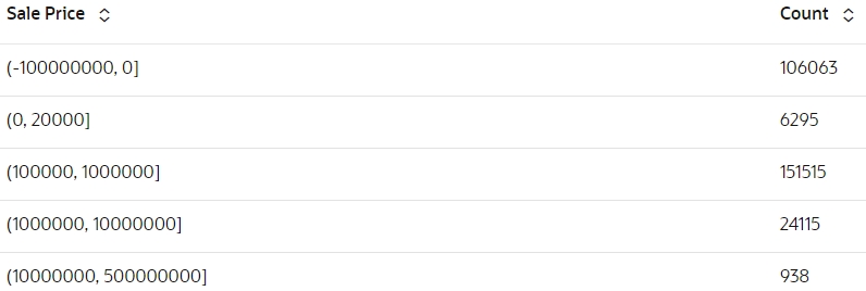 

     
     
     
     
     

   • Examine logarithmic sales price distribution

     
     # Most properties have 10^5 < sale_price < 10^6.5=3.2M
     Nbins = 101
     
     n, bins, patches = plt.hist((BROOKLYN2[BROOKLYN2['sale_price']>0]['sale_price']).log(10).pull(), Nbins)
     plt.xlabel('log10(sale_price)')
     plt.ylabel('number of records')
     p = plt.xlim(3.9, 7.1)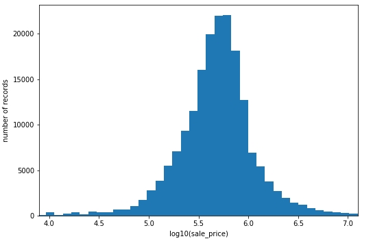

     
     
     
     
     

3. Preview building class category, count and count percentage

   Analyze the categorical column, building_class_category, by computing a cross-tabulation. Sort this table in descending order. Finally, determine the frequency of each building class category.

   build_category= BROOKLYN2.crosstab('building_class_category').sort_values('count', ascending=False)
   count_percentage= ((build_category['count'] / len(BROOKLYN2)) * 100).round(decimals=2)
   z.show(build_category.concat({'count_percentage':count_percentage}))

   
   
   
   
   

4. Examine logarithmic gross qft distribution

   Values in the gross qft column, when log-transformed, approximate a normal distribution.

   # Most properties have 10^2.9=800 < sale_price < 10^3.7=5000
   Nbins = 201
   
   n, bins, patches = plt.hist((BROOKLYN2[BROOKLYN2['gross_sqft']>0]['gross_sqft']).log(10).pull(), Nbins)
   plt.xlabel('log10(sale_price)')
   plt.ylabel('number of records')
   p = plt.xlim(2.5, 4.2)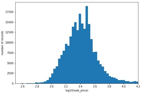

   
   
   
   
   

Feature Engineering

Feature engineering is the process of creating new input features from existing data which explains the underlying patterns of a data. These new featues help to improce the model's predictability.

The following features have been engineered:

• Built Period: The Period in which the house was built.

  built_period=(BROOKLYN2['YearBuilt'] // 10) * 10 + oml.Integer(BROOKLYN2['YearBuilt'] % 10 >= 5) * 10
  BROOKLYN2=BROOKLYN2.concat({'Built_Period':built_period})

• Age_At_Sale: Age of the house at sale is the number of years from its construction to the sale date.

  Age_At_Sale2  = abs(BROOKLYN2['year_of_sale'] - BROOKLYN2['YearBuilt'])
  BROOKLYN2= BROOKLYN2.concat({'Age_At_Sale2': Age_At_Sale2})

• Quarter: Refers to the quarter in which the house was built.

  time_period = oml.Datetime.strptime(BROOKLYN2['sale_date'], format="MM/DD/YYYY")
  Quarter= (oml.Integer((time_period.month - 1)// 3 + 1))

Clean the Dataframe

After feature engineering, remove columns that no longer contribute to the analysis and drop any rows that have a missing value.

BROOKLYN2=BROOKLYN2.drop(['sale_date'])
BROOKLYN2=BROOKLYN2.dropna()

Filter the data to include properties whose sale price, gross square footage, and the decade year of construction fall within a specific, relevant range.

BROOKLYN3 = BROOKLYN2[(BROOKLYN2['sale_price']>=1.0e5) & (BROOKLYN2['sale_price']<=5.0e6) & 
            (BROOKLYN2['gross_sqft']>=800) & (BROOKLYN2['gross_sqft']<=5000) & 
            (BROOKLYN2['Built_Period']>=1900) & (BROOKLYN2['Built_Period']<=2010) ]

Apply a log transformation to normalize the column. The original, untransformed column is then removed.

BROOKLYN3 = BROOKLYN3.concat({'log_gross_sqft': BROOKLYN3['gross_sqft'].log(10)})
BROOKLYN3=BROOKLYN3.drop(['gross_sqft'])

To improve the model's performance, filter the data to focus on properties with higher probabilities of belonging to specific building classes and categories.

BROOKLYN4 = BROOKLYN3[(BROOKLYN3['building_class_at_sale']=='A1') | (BROOKLYN3['building_class_at_sale']=='A2') 
            | (BROOKLYN3['building_class_at_sale']=='A4') | (BROOKLYN3['building_class_at_sale']=='A5') 
            | (BROOKLYN3['building_class_at_sale']=='B1') | (BROOKLYN3['building_class_at_sale']=='B2') 
            |  (BROOKLYN3['building_class_at_sale']=='B3') ]
BROOKLYN5 = BROOKLYN4[((BROOKLYN4['building_class_category']=='02 TWO FAMILY HOMES') | (BROOKLYN4['building_class_category']=='01 ONE FAMILY HOMES'))]

Dataframe Dimensions

Run the following script to verify the dataframe dimensions:

BROOKLYN5.shape

(67083, 32)