@TREND
The @TREND calculation function for Essbase calculates future values based on curve-fitting to historical values.
The @TREND procedure considers a number of observations, constructs a mathematical model of the process based on these observations (that is, fits a curve), and predicts values for a future observation. You can use weights to assign credibility coefficients to particular observations, report errors of the curve fitting, choose the forecasting method to be used (for example, linear regression), and specify certain data filters.
Syntax
@TREND (Ylist, [Xlist], [weightList], [errorList], [XforecastList], YforecastList, method[, method parameters] [, Xfilter1 [, parameters]] [, XfilterN [, parameters]] [, Yfilter1 [, parameters]] [, YfilterN [, parameters]])Parameters
- Ylist
-
An expression list that contains known observations; for example, sales figures over a period of time.
- Xlist
-
Optional. An expression list that contains underlying variable values. For example, for each sales figure in Ylist, Xlist may contain a value for associated time periods. If you do not specify Xlist, the default variable values are 1,2,3, and so on, up to the number of values in Ylist.
- weightList
-
Optional. An expression list that contains weights for the data points in Ylist, for the linear regression method only. If values in weightList are
#MISSING, the default is 1. Weights for methods other than linear regression are ignored. Negative weights are replaced with their absolute values. - errorList
-
Optional. Member list that represents the differences between the data points in Ylist and the data points on the line or curve (as specified for method).
- XforecastList
-
Optional. Expression list that contains the underlying variable values for which the forecasting is sought. If you do not specify XforecastList, the values are assumed to be as follows: {(last value in Xlist + 1), (last value in Xlist + 2), ...}up to (last value in Xlist + the number of values in YforecastList)
If you forecast consecutively from where Ylist stops, you do not need to specify XforecastList. If you want to move the forecasting period forward, specify the new period with XforecastList.
- YforecastList
-
A member list into which the forecast values are placed.
- method
-
A choice among LR (linear regression), SES (single exponential smoothing), DES (double exponential smoothing), and TES (triple exponential smoothing). Method parameters must be numeric values, not member names. Method parameters may be any of the following:
-
LR[,t]: standard linear regression with possible weights assigned to each data point and an optional seasonal adjustment period [t], where [t] is the length of the period. In general, the weights are equal to 1 by default. You might want to increase the weight if the corresponding observation is important, or decrease the weight if the corresponding observation is an outlier or is unreliable.
-
SES[,c]: single exponential smoothing with parameter c (default c=0.2). This method uses its own weight system, using the single parameter c. Increasing this parameter gives more weight to early observations than to later ones.
-
DES[[,c1],c2]: double exponential smoothing (Holt's method) with optional parameters c1, c2 (default c1=0.2, c2=0.3). This is a two-parameter weight system and a linear subsequent approximation scheme. The first parameter controls weight distribution for the intercept; the second parameter controls weight distribution for the slope of the line fit.
-
TES[[[[,T],c1],c2],c3]: triple exponential smoothing (Holt-Winters method) with optional parameters c1, c2, c3, T (default c1=0.2, c2=0.05, c3=0.1, T=1). This is a three-parameter weight system and a linear model with a multiplicative seasonal component.
-
- Xfilter1 ... XfilterN
-
Optional. Use one or more of the following filter methods to scale Xlist:
-
XLOG[,c]: logarithmic change with shift c (x' = log(x+c)) (default c=1)
-
XEXP[,c]: exponential change with shift c (x' = exp(x+c)) (default c=0).
-
XPOW[,c]: power change with power c (x' = x^c) (default c=2).
-
- Yfilter1 ... YfilterN
-
Optional. Use one or more of the following filter methods to scale Ylist:
-
YLOG[,c]: logarithmic change with shift c (y' = log(y+c)) (default c=1)
-
YEXP[,c]: exponential change with shift c (y' = exp(y+c)) (default c=0).
-
YPOW[,c]: power change with power c (y' = y^c) (default c=2).
-
Notes
-
@TREND can be used only in calculation scripts, not in outline formulas.
-
You must associate the @TREND formula with a member.
-
Ylist, Xlist, weightList, and errorList should contain the same number of values.
-
XforecastList and YforecastList should contain the same number of values.
-
The method and filter parameters must be numbers only; functions and member names are not allowed.
-
@TREND ignores
#MISSINGvalues during calculation of the trend. -
When you use the LR method with seasonal adjustments or when you use the TES method, Essbase places strict requirements on the input data. With these methods, input data cannot contain
#MISSINGvalues. Also, if you specify Xlist, the data must be equidistant, with the interval (step) being a whole fraction of the period, T (for example, T/5, T/2). The XforecastList parameters should also contain multiples of the interval. -
For another example using @TREND with more options, see Forecasting Future Values.
-
If you use a member set function to generate a member list for this function, (for example, @SIBLINGS), to ensure correct results, consider the order in which Essbase sorts the generated member list. For more information, see the help topic for the member set function you are using.
-
The following algorithms are used to calculate @TREND:
Algorithm for Linear Regression
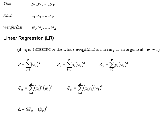
Description of the illustration c_lr1_1.gif
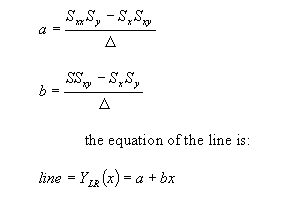
Description of the illustration c_lr1_2.gif
Algorithm for Linear Regression with Seasonal Adjustment
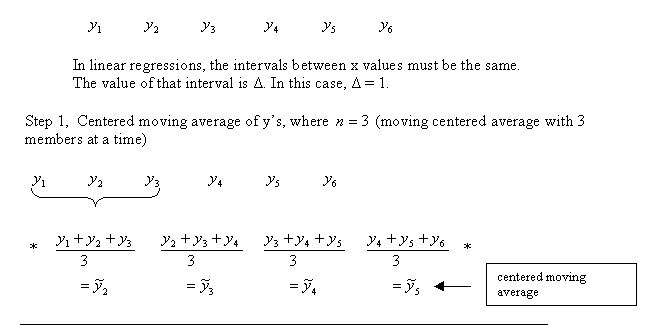
Description of the illustration c_des_3.gif
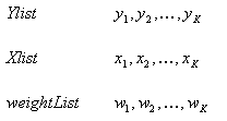
Description of the illustration c_lr2_1.gif
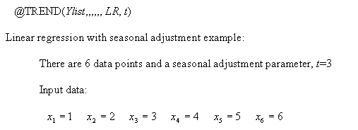
Description of the illustration c_lr2_2.gif
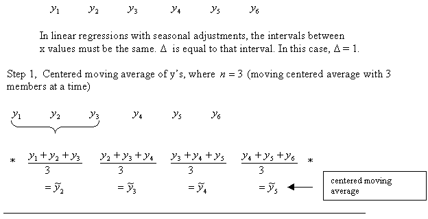
Description of the illustration c_lr2_3.gif
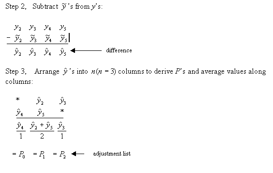
Description of the illustration c_lr2_4.gif
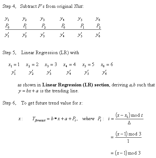
Description of the illustration c_lr2_5.gif
Algorithm for Single Exponential Smoothing (SES)

Description of the illustration c_ses_1.gif
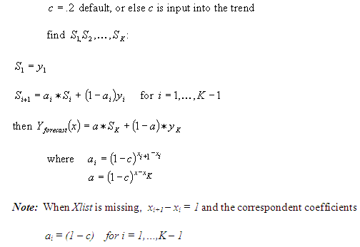
Description of the illustration c_ses_2.gif
Algorithm for Double Exponential Smoothing (DES)

Description of the illustration c_des_1.gif
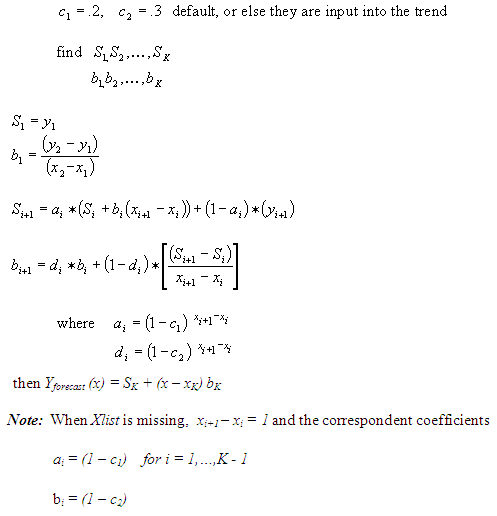
Description of the illustration c_des_2.gif
Algorithm for Triple Exponential Smoothing (TES)

Description of the illustration c_tes_1.gif
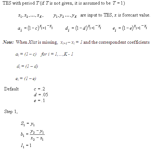
Description of the illustration c_tes_2.gif
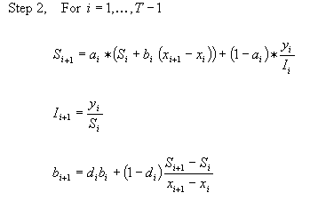
Description of the illustration c_tes_3.gif
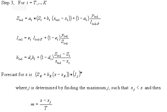
Description of the illustration c_tes_4.gif
Example
The following example is based on the Sample Basic database. It forecasts sales data for May through December, based on the trend of the same sales data from January through April. The method used is linear regression with no seasonal adjustment.
Sales(@TREND(Jan:Apr,,,,,May:Dec,LR););This example produces the following report:
           Actual    Sales    West
                     Colas
                     =====
Jan                   2339
Feb                   2298
Mar                   2313
Apr                   2332
May                   2319
Jun                   2318.4
Jul                   2317.8
Aug                   2317.2
Sep                   2316.6
Oct                   2316
Nov                   2315.4
Dec                   2314.8
  Year               27817.2
See Also