3.3.2 Explore Data
Explore the data to understand its structure and assess its quality. At this stage, identify the data types and detect any noise present. Check for missing values as well as numeric outliers.
Note:
Each record in the database is called a case, and each case is identified by a case_id. Here, the case id is TIME_ID, which serves as the independent variable. You are forecasting sales over evenly spaced time intervals.
The following steps will guide you through exploratory data analysis.
-
Import libraries
Run the following command in an R interpreter paragraph (using %r) in a notebook to import the Oracle Machine Learning for R libraries and suppress warnings regarding row ordering. This establishes a default connection to the database for use by OML4R.Note:
The OML4R functions are prefixed with "ore," which refers to the original product name "Oracle R Enterprise."library(ORE) options(ore.warn.order=FALSE) -
Create a DataFrame proxy object on the SH.SALES table
Use the
This script uses the ore.sync function to create a data.frame proxy object to the table SH.SALES in the object ESM_SALES. It then attaches the synchronized object to the R environment withore.syncfunction to create the a proxy objectESM_SALESfor theSH.SALESdatabase table. Theore.syncfunction returns anore.frameobject that represents the table in OML4R.ore.attach(), allowing direct access toESM_SALESas if it were a local data frame. Finally, it displays the first few rows of this data usinghead()combined with ORE’s formatted output functionz.show().ore.sync(query = c(ESM_SALES = "select * from SH.SALES")) ore.attach() z.show(head(ESM_SALES))The output appears as follows:

This output displays the first 6 rows of the
SH.SALESdatabase table, including all available columns. It allows you to quickly inspect a sample of the sales data stored in the Oracle database directly from your OML4R session. -
Sales dataset row and column count
To determine the number of rows and columns in the
ore.frameobjectSALES, use the functiondim(SALES).This script runs an R command inside a notebook to return the number of rows and columns of the
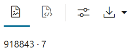
ESM_SALESdata frame or table.%r dim(ESM_SALES)
The output shows the number of rows and columns in the
ESM_SALESdataset to understand the shape and scale of the data you are working with in OML4R. -
Sales Dataset Column Types
Use the following code to view the data type of each column.
This script retrieves and displays metadata for the
ESM_SALESobject in OML4R, providing details about the structure and columns of the linked Oracle database table.
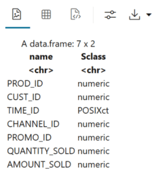
The output appears as follows:%r ESM_SALES@desc
The output of
ESM_SALES@descis a structure of theESM_SALESobject. It includes Column names and Data types. -
Count of missing values by column
To check if there are any missing values in the data, run the following code. It returns you the total number of missing values in the
ESM_SALESproxy object to assess data completeness.%r sum(is.na(ESM_SALES))The output appears as 0, which indicates that there are no missing values in the
ESM_SALESproxy object. -
Prepare the data for sales forecasting, start by selecting the required columns from the
SH.SALEStable.Use the
ore.sync()function to create a proxy object namedSALES_TIME_AMOUNTcontaining theTIME_IDandAMOUNT_SOLDcolumns..This defines a new
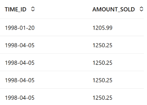
ore.data.frameobject in R calledSALES_TIME_AMOUNTby linking it to a query that selectsTIME_IDandAMOUNT_SOLDcolumns from theSH.SALEStable in an Oracle database. It helps in-database analytics without fully loading the data into R.%r ore.sync(query = c(SALES_TIME_AMOUNT = "select TIME_ID, AMOUNT_SOLD from SH.SALES")) z.show(head(SALES_TIME_AMOUNT))) The output shows the formatted table with the first 6 rows of the SALES_TIME_AMOUNT dataset. It includes two columns:
- TIME_ID – A time identifier (date).
- AMOUNT_SOLD – A numeric value showing the amount sold for each transaction.
-
Use the
dim()function to view the dimensions (number of rows and columns) of theSALES_TIME_AMOUNTproxy object. This helps confirm the size of the dataset retrieved from theSH.SALEStable.The returns the number of rows and columns in the
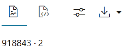
SALES_TIME_AMOUNTdataset, showing you the shape of the data queried from the database.%r dim(SALES_TIME_AMOUNT)
The output of
dim(SALES_TIME_AMOUNT)shows that the dataset contains 918843 rows and 2 columns. This gives you a quick understanding of the dataset’s size and structure.
This gives you a quick understanding of the dataset’s size and structure.
Parent topic: Time Series Use Case