Explore Data

3.2.2 Explore Data

Once the data is accessible, explore the data to understand and assess the quality of the data. At this stage assess the data to identify data types and noise in the data. Look for missing values and numeric outlier values.

To gain a broader understanding of the data and identify potential issues, we will now explore the dataset, focusing on data quality assessment and identifying missing or outlier values.

To determine the number of rows and columns in the ore.frame object CUSTOMERS, use dim(CUSTOMERS).
```
dim(CUSTOMERS)
55500    6
```
To determine the number of rows and columns in the ore.frame object SUPPLEMENTARY_DEMOGRAPHICS, use dim(SUPPLEMENTARY_DEMOGRAPHICS)
```
dim(SUPPLEMENTARY_DEMOGRAPHICS)
4500   4
```
Create a new ore.frame object CUST_DF by merging the table CUSTOMERS and SUPPLEMENTARY_DEMOGRAPHICS with an inner join on the common column CUST_ID. The merge function joins one ore.frame to another ore.frame.
```
CUST_DF <- merge(SUPPLEMENTARY_DEMOGRAPHICS,CUSTOMERS, by="CUST_ID")
```
To display first 5 rows of CUST_DF data run the following code:
```
z.show(head(CUST_DF,5))
```
To get the dimensions using CUST_DF proxy object, use 'dim':
```
dim(CUST_DF)
 
   4500   9
```

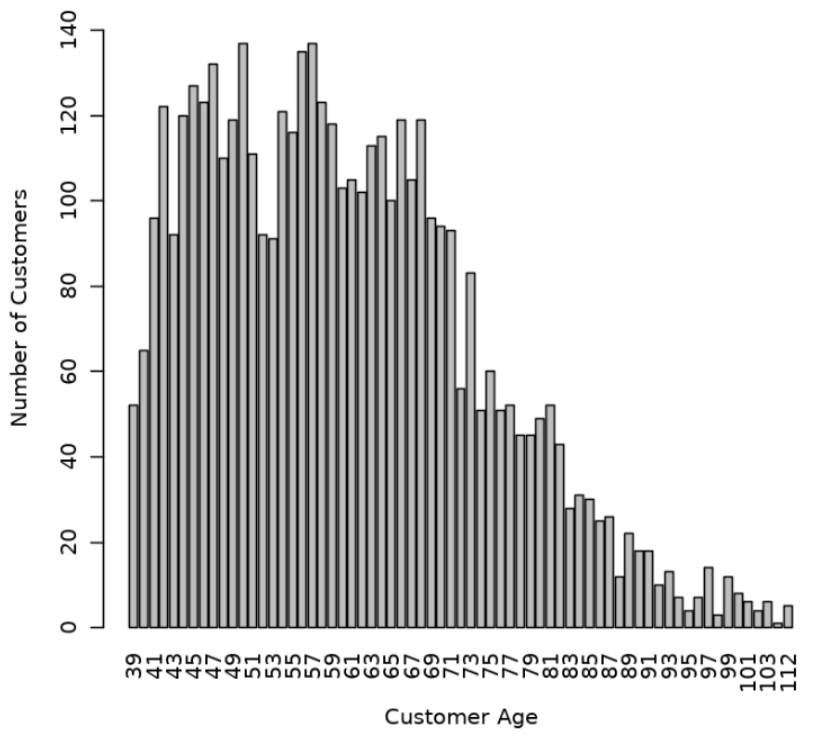
To transform the column CUST_YEAR_OF_BIRTH to CUST_AGE in the CUST_DF proxy object and produce a barplot of the distribution of customer ages, use the following code.

Date1 <- format(Sys.Date(), "%Y")
Date2 <- as.numeric(Date1)
CUST_DF$CUST_AGE <- Date2-CUST_DF$CUST_YEAR_OF_BIRTH
CUST_DF$CUST_YEAR_OF_BIRTH <- NULL
tbl <- with(CUST_DF, table(CUST_AGE))
barplot(tbl, ylim=c(0,150), ylab = "Number of Customers", xlab = "Customer Age", las=3)

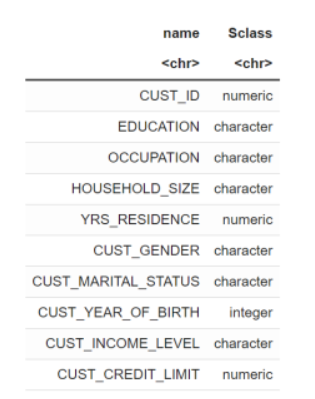
This image shows the bar plot of the distribution of customer ages.

View the data type of the columns in CUST_DF with the @desc operator, which is crucial for understanding to understand your data and perform calculations accurately.
```
CUST_DF@desc
```
To check if there are any missing values in the data, run the following code. The following code gives you the total number of missing values in the CUST_DF proxy object.
```
sum(is.na(CUST_DF))
0
```
The value 0 indicates that there are no missing values in the CUST_DF proxy object.
Use the crosstab method to perform a cross-column analysis of the ore.frame object in the database. By default, it computes a frequency table for the columns unless a column and an aggregation function have been passed to it. In this example, the crosstab function displays the distribution of unique values of CUST_CREDIT_LIMIT along the x-axis and its occurrence frequency along the y-axis.
In the output, click the Bar chart. In the Settings tab, choose “CUST_CREDIT_LIMIT” as the Group By column, and use “Last” as the Aggregate Duplicates function.
```
ct <- ore.crosstab(~CUST_CREDIT_LIMIT, data=CUST_DF)
z.show(ct)
```

To compute the statistics of the CUST_DF table, use the summary function.

options(width = 80)
summary(subset(CUST_DF, select = -CUST_ID))
   
CUST_GENDER            CUST_MARITAL_STATUS    CUST_INCOME_LEVEL    
 Length:4500            Length:4500            Length:4500          
 Class :ore.character   Class :ore.character   Class :ore.character 
 Mode  :character       Mode  :character       Mode  :character     
                                                                      
                                                                      
                                                                      
 CUST_CREDIT_LIMIT HOUSEHOLD_SIZE         YRS_RESIDENCE     Y_BOX_GAMES   
 Min.   : 1500     Length:4500            Min.   : 0.000   Min.   :0.0000 
 1st Qu.: 5000     Class :ore.character   1st Qu.: 3.000   1st Qu.:0.0000 
 Median : 9000     Mode  :character       Median : 4.000   Median :0.0000 
 Mean   : 7924                            Mean   : 4.022   Mean   :0.3124 
 3rd Qu.:11000                            3rd Qu.: 5.000   3rd Qu.:1.0000 
 Max.   :15000                            Max.   :14.000   Max.   :1.0000 
    CUST_AGE    
 Min.   : 39.00 
 1st Qu.: 49.00 
 Median : 59.00 
 Mean   : 60.38 
 3rd Qu.: 69.00 
 Max.   :112.00

This completes the data understanding stage.

Data Preparation

Before building the model you want to clean the data, if needed. Usually, data can contain outliers that may form a separate cluster, which can affect model quality. The command below defines the function filter_outliers to calculate the interquartile range for a dataframe object. The function remove_outliers uses a for loop to compute the interquartile range for the list of features. The user-defined function remove_outliers uses the interquartile range to find outliers in the data and remove them.

# create filter outliers function
filter_outliers <- function(x) {
  
    # calculate first quantile
    Quantile1 <- quantile(x, probs=.25)
  
    # calculate third quantile
    Quantile3 <- quantile(x, probs=.75)
  
    # calculate inter quartile range
    IQR = Quantile3-Quantile1
  
    # return true or false
    x < Quantile3 + (IQR*1.5) & x > Quantile1 - (IQR*1.5)
}
 
# create remove outliers function
remove_outliers <- function(dataframe,
                            columns=names(dataframe)) {
  
    # for loop to traverse in columns vector
    for (col in columns) {
  
        # remove observation if it satisfies outlier function
        dataframe <- dataframe[filter_outliers(dataframe[[col]]),]
    }
    ore.pull(dataframe)
}
  
CUST_DF_CLEAN <- remove_outliers(CUST_DF, c('CUST_AGE', 'CUST_CREDIT_LIMIT', 'YRS_RESIDENCE', 'Y_BOX_GAMES'))
CUST_DF_CLEAN <- ore.push(CUST_DF_CLEAN)
dim(CUST_DF_CLEAN)

4233 9

This completes the data preparation stage.

Parent topic: Clustering Use Case