Information about Model settings

Evaluate the model by examining the various statistics generated after building the model. The statistics indicate the model's quality.

• Model details: Run the following script for model details available through the GLM model object, like the model settings, attribute coefficients, fit details, etc.

  glm_mod

  They can also be displayed and viewed individually as shown below.

• Attribute Coefficient: Run the following script to display the model's attribute coefficient.

  z.show(glm_mod.coef.round(2).head())

  
  
  
  
  
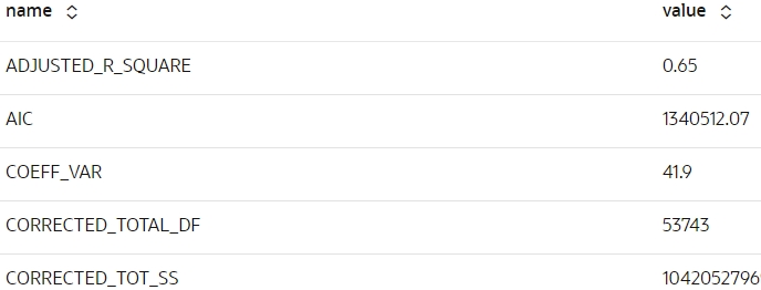
• Fit Details: Run the following script to display the fit details of the model.

  z.show(glm_mod.fit_details.round(2).head())

  
  
  
  
  

Score

Scoring is the process of applying the model on the test data to access its performance.

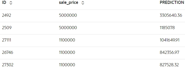
1. Predict sale price: Use the model to make predictions on test data.

   BROOKLYN_RES = glm_mod.predict(TEST.drop('sale_price'), supplemental_cols = TEST[:,['ID','sale_price']])
   z.show(BROOKLYN_RES.round(2).head())

   
   
   
   
   
2. Evaluate Model Performance: Evaluate the model's performance by using the score function.

   model_coef = len(glm_mod.coef)
   no_rows_test = TEST_X.shape[0]
   R_squared = glm_mod.score(TEST_X, TEST_Y).round(3)
   
   print(
       f"RMSE : {(((BROOKLYN_RES['PREDICTION'] - BROOKLYN_RES['sale_price']) ** 2).mean() ** .5).round(2)}\n"
       f"MAE: {((abs(BROOKLYN_RES['PREDICTION'] - BROOKLYN_RES['sale_price'])).mean()).round(2)}\n"
       f"R squared: {R_squared}\n"
       f"Adjusted R^2: {(1 - ( 1 - R_squared)*(no_rows_test-1)/(no_rows_test - model_coef -1)).round(4)}"
   )

   The interpreation of the model's performance based on the metrics are as follows:

   • RMSE (286,137.56): The model's predictions, on average, deviate by approximately 286,137.56 units from the actual values.
   • MAE (170,992.05): The average absolute error in predictions is 170,992.05 units, which provides a sense of the model's accuracy without penalizing large errors.
   • R² (0.581): The model explains 58.1% of the variance in the target variable, suggesting a moderate fit to the data.
   • Adjusted R² (0.5604): After adjusting for the number of predictors, the model explains about 56.04% of the variance

   Overall, the model demonstrates moderate predictive accuracy, with potential for further improvement.

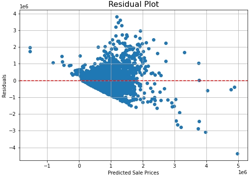
3. Residual Graph: The Residual plot is showing heteroscedastic pattern. This indicates that the errors in the model are inconsistent. The non-linear relationship between the fitted values (predicted values) and the residuals, suggests that the model can be improved further.

   import matplotlib.pyplot as plt
    
   y_pred = BROOKLYN_RES['PREDICTION'].pull()
   residuals = (BROOKLYN_RES['sale_price'] - BROOKLYN_RES['PREDICTION']).pull()
    
   plt.scatter(y_pred, residuals)
    
   plt.xlabel('Predicted Sale Prices')
   plt.ylabel('Residuals')
   plt.title('Residual Plot', fontsize=16)
   plt.grid(True)
   plt.axhline(y=0, color='r', linestyle='--')
   plt.show()

   
   
   
   
   

SQL Interface to Score Data and Display Prediction Details

You can score data and make predictions using the SQL interface. The test data is materialized into BROOKLYN_GLM_TEST_DATA so that you can query it using SQL. The materialized method writes the contents of an Oracle Machine Learning oml.DataFrame proxy table to an Oracle Database table.

1. Materialize BROOKLYN_GLM_TEST_DATA for use in query below:

   try:
       oml.drop(table = 'BROOKLYN_GLM_TEST_DATA')
   except:
       pass
   _ = TEST.materialize(table = 'BROOKLYN_GLM_TEST_DATA')

2. Display prediction with explanatory prediction details in SQL: The SQL command to score and display the prediction details. The prediction functions apply a glm regressional model named BROOKLYN_GLM_REGRESSION_MODEL to the data from the materialized table BROOKLYN_GLM_TEST_DATA. The query includes information about the predictors that have the greatest influence on the prediction.

   SELECT ID,
          round(PREDICTION_YRS_RES,3) PRED_YRS_RES,
          round(PRED_LOWER_LIMIT,1) LOWER_BOUND,
          round(PRED_UPPER_LIMIT,1) UPPER_BOUND,
          RTRIM(TRIM(SUBSTR(OUTPRED."Attribute1",17,100)),'rank="1"/>') FIRST_ATTRIBUTE,
          RTRIM(TRIM(SUBSTR(OUTPRED."Attribute2",17,100)),'rank="2"/>') SECOND_ATTRIBUTE,
          RTRIM(TRIM(SUBSTR(OUTPRED."Attribute3",17,100)),'rank="3"/>') THIRD_ATTRIBUTE
   FROM (SELECT ID,
                PREDICTION(BROOKLYN_GLM_REGRESSION_MODEL USING *) PREDICTION_YRS_RES,
                PREDICTION_BOUNDS(BROOKLYN_GLM_REGRESSION_MODEL USING *).LOWER PRED_LOWER_LIMIT,
                PREDICTION_BOUNDS(BROOKLYN_GLM_REGRESSION_MODEL USING *).UPPER PRED_UPPER_LIMIT,
                PREDICTION_DETAILS(BROOKLYN_GLM_REGRESSION_MODEL USING *) PD
         FROM BROOKLYN_GLM_TEST_DATA
         WHERE ID < 100015
         ORDER BY ID) OUT,
        XMLTABLE('/Details'
                 PASSING OUT.PD
                 COLUMNS 
                 "Attribute1" XMLType PATH 'Attribute[1]',
                 "Attribute2" XMLType PATH 'Attribute[2]',
                  "Attribute3" XMLType PATH 'Attribute[3]') OUTPRED