3.3.2 Explore Data
Once the data is accessible, explore the data to understand and assess the quality of the data. At this stage assess the data to identify data types and noise in the data. Look for missing values and numeric outlier values.
Assess Data Quality
To access database data from Python using OML4Py, you must first create a
oml.DataFrame proxy object in Python which represents a
database table, view, or query. Create a oml.DataFrame proxy object
for SUPPLEMENTARY_DEMOGRAPHICS and CUSTOMERS and then merge them by inner join on a
key column, e.g., CUST_ID. Assess the data to identify data types
and noise in the data. Look for missing values, outlier numeric values, or
inconsistently labeled categorical values.
The following steps help you with the exploratory analysis of the data:
- Run the following script in a
%pythoninterpreter paragraph to import theomlmodules, the Panda's module, and set the display options:import pandas as pd import matplotlib.pyplot as plt import oml pd.set_option('display.max_rows', 500) pd.set_option('display.max_columns', 500) pd.set_option('display.width', 1000) import warnings warnings.simplefilter(action='ignore', category=FutureWarning) - Use the
oml.syncfunction to create the Python object DEMOGRAPHICS as a proxy for a database table SUPPLEMENTARY_DEMOGRAPHICS. Theoml.syncfunction returns anoml.DataFrameobject. Theoml.DataFrameobject returned byoml.syncis a proxy for the database object.Note:
Only one environment for a given database schema can exist at a time. If"schema=None", then objects are created searched in the current user's schema.DEMOGRAPHICS = oml.sync(table = "SUPPLEMENTARY_DEMOGRAPHICS", schema = "SH") z.show(DEMOGRAPHICS.head())
- To determine the number of rows and columns in the
oml.DataFrameobject DEMOGRAPHICS, useDataFrame.shape.print("Shape:",DEMOGRAPHICS.shape)(4500, 14) - Use the
oml.syncfunction to create the Python object CUSTOMERS as a proxy for a database table SH.CUSTOMERS. The query argument uses the SQL SELECT statement for selecting columns to include for use through the proxy object.cCUSTOMERS = oml.sync(query = 'SELECT CUST_ID, CUST_GENDER, CUST_MARITAL_STATUS, CUST_YEAR_OF_BIRTH, CUST_INCOME_LEVEL, CUST_CREDIT_LIMIT FROM SH.CUSTOMERS') z.show(CUSTOMERS.head())
- To determine the number of rows and columns in the
oml.DataFrameobject CUSTOMERS, useDataFrame.shape.print("Shape:",CUSTOMERS.shape)(55500, 6) - Create a new
oml.DataFrameCUSTOMER_DATA by merging the table CUSTOMERS and DEMOGRAPHICS with an inner join on the common column CUST_ID. The merge function joins one oml.DataFrame to another oml.DataFrame. The suffixes parameter is used when the two oml.DataFrame have conflicting column names.CUSTOMER_DATA = CUSTOMERS[["CUST_ID", "CUST_GENDER", "CUST_MARITAL_STATUS", "CUST_YEAR_OF_BIRTH", "CUST_INCOME_LEVEL", "CUST_CREDIT_LIMIT"]].merge(DEMOGRAPHICS[["CUST_ID", "HOUSEHOLD_SIZE","YRS_RESIDENCE", "Y_BOX_GAMES"]], how = "inner", on = 'CUST_ID',suffixes = ["",""]) - To determine the number of rows and columns in the
oml.DataFrameobject CUSTOMER_DATA, use DataFrame.shape.print("Shape:",CUSTOMER_DATA.shape)Shape: (4500, 9) - Use the
concatfunction to concatenate the new column CUST_AGE in anoml.DataFrameobject CUSTOMER_DATA. The column CUST_AGE contains the age based on the column CUST_YEAR_OF_BIRTH where the year of birth is converted to age in the year 2005. The information in the CUST_YEAR_OF_BIRTH column has been modified and maintained in CUST AGE, so drop the CUST_YEAR_OF_BIRTH column.CUSTOMER_DATA=CUSTOMER_DATA.concat({'CUST_AGE':abs(CUSTOMER_DATA['CUST_YEAR_OF_BIRTH'] -2005)}) CUSTOMER_DATA=CUSTOMER_DATA.drop('CUST_YEAR_OF_BIRTH') CUSTOMER_DATA.head()
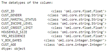
- Run the following script to view the data type of each
column.
print("The datatypes of the column: ","\n")
print(CUSTOMER_DATA.dtypes)
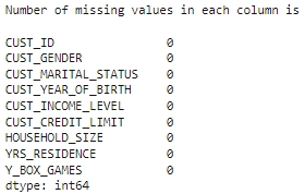
- To check if there are any missing values run the following script.
The count function returns the number of elements that are not NULL for each
column and the
len()function returns the number of rows in the dataset.print("Number of missing values in each column is : \n") print(len(CUSTOMER_DATA)-CUSTOMER_DATA.count())
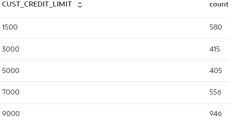
- Use the crosstab method to perform a cross-column analysis of an
oml.DataFrameobject in the database. The crosstab method computes a cross-tabulation of two or more columns. By default, it computes a frequency table for the columns unless a column and an aggregation function have been passed to it. In this example, the crosstab function displays the distribution of unique values of CUST_CREDIT_LIMIT along the x-axis and its occurrence frequency along the y-axis.z.show(CUSTOMER_DATA.crosstab(‘CUST_CREDIT_LIMIT’))
- Use the transparency layer method
describeto calculate descriptive statistics that summarize the central tendency, dispersion, and shape of the CUSTOMER_DATA table in each numeric column.Note:
All computations are computed in the database and only the result statistics are returned to the Python client, in this case, the notebook. Eliminating the need to move data and using the database as a high-performance compute engine greatly increases scalability.CUSTOMER_DATA.describe()
- Before building the model, it's important to ensure that the data
is clean. Data often contains outliers, which can form separate clusters that
negatively impact model quality.
The following script defines a function, IQR, to calculate the interquartile range for a dataframe. It takes two arguments: SUMMARY_DF (which contains summary statistics of the dataframe, generated using the
Run the script to calculate the interquartile range for the specified columns:describemethod) and a list of features. The IQR function uses a for loop to compute the interquartile range for each feature in the list.def IQR(SUMMARY_DF, features): result = [0]*len(features) for i, feature in enumerate(features): result[i] = abs(SUMMARY_DF[feature]['75%'] - SUMMARY_DF[feature]['25%']) return result print(IQR(CUSTOMER_DATA.describe(),['CUST_AGE', 'CUST_CREDIT_LIMIT', 'YRS_RESIDENCE', 'Y_BOX_GAMES']))[20.0, 6000.0, 2.0, 1.0]The user-defined function
The following function removes rows with outliers of a given feature based on quantiles:remove_outlieruses the interquartile range to find outliers in the data and remove them. In boxplot, outliers are points that lie outside of the upper and lower quartiles by 1.5 times the interquartile range (Q1 - 1.5 * IQR or Q3 + 1.5 * IQR). Another form of outlier treatment is clipping or capping, where more extreme values are replaced with a max or min value, e.g., the 1.5 IRQ values.def remove_outlier(DF, SUMMARY_DF, features): iqrs = IQR(SUMMARY_DF, features) for i, iqr in enumerate(iqrs): H = 1.5*iqr DF = DF[ ( DF[features[i]] > SUMMARY_DF[features[i]]['25%'] - H ) & ( DF[features[i]] < SUMMARY_DF[features[i]]['75%'] + H )] print(DF.shape) return DF CUSTOMER_DATA_CLEAN= remove_outlier(CUSTOMER_DATA, CUSTOMER_DATA.describe(), ['CUST_AGE', 'CUST_CREDIT_LIMIT', 'YRS_RESIDENCE', 'Y_BOX_GAMES']) print("Shape:",CUSTOMER_DATA_CLEAN.shape)Shape: (4233, 9)
This completes the data understanding and data preparation stage.
Parent topic: Clustering Use Case