DBSCAN is a density-based clustering technique capable of finding clusters of different shapes and sizes from a large amount of data.

This algorithm does not require the number of clusters as a parameter. Instead, it uses the following parameters.

• min_samples: The minimum number of points required for a region to be considered a cluster.
• eps: The distance threshold for searching points in the neighborhood of a point.

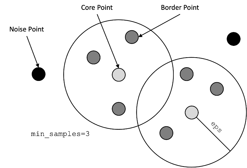
The algorithm starts at any point. If at least min_samples points are within a radius of eps, then all the points in the neighborhood are considered part of the same cluster. The process is then repeated for all the points in the neighborhood. There are three types of points or observations:

• Core Point: At least has a min_samples number of points in its neighborhood within the radius eps.
• Border Point: It is reachable from a core point, but there are fewer than min_samples number of points within its neighborhood.
• Noise Point: It is neither a core point nor a border point. It is a point that is not reachable from any core points.

The following image is an example displaying the different types in the DBSCAN algorithm.

Standard DBSCAN clustering does not fully consider the observation’s spatial location. When this algorithm is applied on spatial data, it often results in data points of a cluster dispersed across spatial regions. Regionalization is used to provide a spatial context to the DBSCAN algorithm, this way, observations of the same cluster are similar not only in their attributes, but also in their spatial location.

The DBSCAN algorithm with regionalization performs the following steps:

1. Creates an instance of the DBScanClustering class specifying the parameters: min_samples, eps, and spatial_weights_definition.
2. Calls the fit method passing the data as parameter to train the model.
3. The labels_ property indicates the label assigned to each observation. Noise points are labeled with -1. Use the labels and the location of each observation to visualize the clusters in a map.

If you do not provide the eps parameter, it is estimated automatically (see [1] for more details on eps estimation method). The initial eps value is estimated by:

• Calculating the Euclidean distance between each pair of neighboring locations using the K-nearest neighbors approach, where the value of k is equal to min_samples.
• Obtaining the distance to the nearest neighbor for each observation and sorting the distances in ascending order.
• Plotting the sorted distances to form an elbow curve.
• The estimated value of eps is the distance associated with the elbow's location, which is represented by the furthest point from the line that crosses the first and last points.

See the DBScanClustering class in Python API Reference for Oracle Spatial AI for more information.

The following code fits a DBSCAN model with training data from the block_groups SpatialDataFrame. The goal is to identify geographic areas with similar characteristics.

The clustering model is the final step of a spatial pipeline, which contains a preprocessing step to standardize the data. The geometry column is not considered a feature but it is used to compute the spatial weights.

from oraclesai.weights import KNNWeightsDefinition 
from oraclesai.clustering import DBScanClustering 
from oraclesai.pipeline import SpatialPipeline 
from sklearn.preprocessing import StandardScaler 
 
# Define variables and CRS 
X = block_groups[['MEDIAN_INCOME', 'MEAN_AGE', 'MEAN_EDUCATION_LEVEL', 'geometry']].to_crs('epsg:3857') 
 
# Create an instance of DBScanClustering
reg_dbscan = DBScanClustering(eps=0.9,  
                              min_samples=5,  
                              spatial_weights_definition=KNNWeightsDefinition(k=30)) 
 
# Add the model into a Spatial Pipeline with a preprocessing step
reg_dbscan_pipeline = SpatialPipeline([('scale', StandardScaler()), ('clustering', reg_dbscan)]) 
 
# Train the model
reg_dbscan_pipeline.fit(X) 
 
# Print the labels
print(f"labels = {reg_dbscan_pipeline.named_steps['clustering'].labels_[:20]}")

The preceding code prints the label assigned to the first 20 observations using the DBSCAN algorithm with regionalization.

labels = [ 0  0  0  0  0  0  0 -1  0  0  0  0  0 -1  0  0  0  0  0  0]