clustering

Format

clustering(table, method, scale=True, key_column=None, columns=None, weights=None, weights_def=None,
   save_weights_as=None, spatial_col=None, crs=None, to_crs=None, plot=None, **kwargs)

Parameters

The parameters for this pre-defined function are described in the following table.

Parameter	Description
`method`	A string specifying the clustering algorithm to execute. The options are: DBSCAN, KMEANS ,and AGGLOMERATIVE.
`scale`	If specified, it calls the function `oml.create` to store a pandas `DataFrame` containing spatial lag in a table with the specified name.
`key_column`	If defined, the specified column is added to the resulting pandas `DataFrame`. Otherwise, a column with the index of the `DataFrame` is attached to the result.
`columns`	An array of strings indicating the features that form the training set.
`weights`	Required when trying to use spatial weights already stored in the data store. Internally it calls the function `olm.ds.load`. The supported parameters are `ds_name` and `obj_name`, indicating the data store name and object name, respectively.
`weights_def`	Required if the parameter `weights` is not specified. Establishes the relationship between neighboring locations. This is passed as a json object specifying the type of the weights definition and its parameters. Each parameter is defined in detail in the API Reference documentation. The following lists the supported types and parameters: KNN: `[k]` Kernel: `[bandwidth, fixed, k, function]` DistanceBand: `[threshold, p, alpha, binary]` Queen Rook
`save_weights_as`	Only used if `weights_def` is defined. Specifies how the spatial weights are stored in the data store. The value is a json file that determines the parameters of `oml.ds.save`. The supported parameters are: `[ds_name, obj_name, overwrite_ds, append, overwrite_obj, grantable, compression]`. Some parameter names slightly differ from those in the `oml.ds.save` function. The parameter `overwrite_obj` is used to indicate whether an already existing object should be replaced with the current object.
`spatial_col`	Specifies the column containing the geometries. The column can be specified in the table’s metadata. If not specified, the column name is retrieved from the table.
`crs`	Specifies the Coordinate Reference System. If not specified, it is inferred from the table.
`to_crs`	If specified, the Coordinate Reference System will change to the specified value.
`plot`	A dictionary specifying the properties of the Plot Clusters function. If defined, a plot showing the resulting clusters is included in the response.

Example

This example shows how to run the agglomerative with regionalization algorithm over a given dataset, specifying the number of clusters and the type of spatial weights.

The clustering algorithm is set in the method parameter, while the number of clusters and the spatial weights are defined in the n_clusters and weights_def parameters respectively. The features considered for clustering are specified in the columns parameter.

select *
    from table( 
        pyqEval(
            '{  
                "oml_connect": true, 
                "table": "oml_user.la_block_groups",
                "columns": ["median_income"],
                "method": "AGGLOMERATIVE",
                "n_clusters": 6,
                "key_column": "geoid",
                "weights_def": {"type": "Queen"}
            }',
            '{ "geoid": "VARCHAR2(50)", "label": "NUMBER" }',
            'clustering'
        )
    );

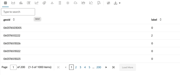
The result contains the index column specified in the key_column parameter and the labels of each row, indicating to which cluster they belong.

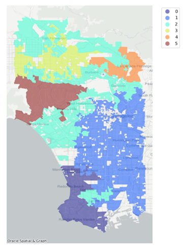
Description of the illustration clustering.png

You can visualize the clusters using the select IMAGE clause and the oml_graphics_flag parameter set to true. In the following code, the plot parameter indicates that it uses a basemap as background. Also, note that the output format (out_fmt) is set to PNG.

select IMAGE
    from table(
        pyqEval(
            par_lst => '{
            "oml_connect": true,
            "oml_graphics_flag": true,
            "table": "oml_user.la_block_groups",
            "columns": ["median_income"],
            "method": "AGGLOMERATIVE",
            "n_clusters": 6, 
            "key_column": "geoid",
            "weights_def": {"type": "Queen"},
            "plot": {"with_basemap": true}
        }',
        out_fmt => 'PNG',
        scr_name => 'clustering'
    )
);

The result is a map with the observations colored according to the cluster they are assigned. Note that there are six clusters as specified in the n_clusters parameter. By defining spatial weights, the agglomerative clustering algorithm executes regionalization. This means that observations assigned to the same cluster share common characteristics and are geographically connected.

Description of clustering_viz.png follows

Description of the illustration clustering_viz.png